Advanced Graphics

Examples class 3

• [2009 P7 Q2] State the Jordan curve theorem [1 mark]. Given point V and simple convex planar polygon P in , express:
  • A test for whether V is coplanar with P. [1 mark]
  • A test for whether V lies strictly inside P. [2 marks]
  • A test for whether V lies on the border of P. [1 mark]

• What is the angle deficit of a vertex, AD(v)? [2 marks]
  Given a closed orientable polyhedral surface of genus g, what is the sum, AD(v), of the angle deficits for all vertices on the surface? [3 marks]

• Various bounding volumes can be used to accelerate intersection tests. In what circumstances would it be appropriate to use:
  • axis-aligned bounding boxes?
  • oriented bounding boxes?
  • bounding spheres?
  [5 marks]

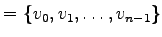
• [2005 P7 Q3] Brian and Geoff Wyvill developed a blobby object modelling method where the blobby object is defined by a number, n, of centres, , each with an associated radius, . They define a function

  (1)

  
  
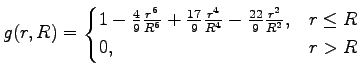
  and sum the contributions from all centres to give a function over all space

  (2)

  
  
  The surface of the blobby object is defined as all points, , where

  (3)

  
  
  Sketch, in 2D, the 2D blobby ``surface'' for each of the following cases:
  • n = 2, = (0, 0), = 2, = (4, 0), = 2; [2 marks]
  • n = 2, = (0, 0), = 2, = (2, 0), = 2; [2 marks]
  • n = 2, = (0, 0), = 2, = (3, 0), = 4; [2 marks]
  Describe variations of equation (2) which allow for:
  • CSG union of blobby objects; [1 mark]
  • CSG intersection of blobby objects; [1 mark]
  • CSG difference of blobby objects. [2 marks]

• An approximate polygonization is used to visualize the isosurface (such as an implicit, `blobby' surface) of a 3D field. The most popular methods for constructing this polygonization operate on volumetric cubes, but these can introduce `ambiguous' cases which prevent the construction of a watertight polygonization. Briefly describe methods which are available to guarantee a watertight polygonization:
  • without using additional samples from the 3D field (required when visualising MRI data, for example); [3 marks]
  • when it is possible to sample the field at new positions (when blobby modelling, for example). [3 marks]

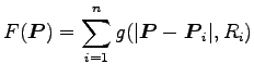
• The function renderSquare() executes OpenGL commands to draw a square with vertices at (-1, -1), (-1, 1), (1, 1) and (1, -1). Sketch the shape drawn in the xy-plane by the following sequence of OpenGL commands: [4 marks]

  glPushMatrix();
    glTranslatef(1, 1, 0);
    glPushMatrix();
      glRotatef(45, 0, 0, 1);
      renderSquare();
    glPopMatrix();
    renderSquare();
  glPopMatrix();
  

  Show how the above sequence should be modified to produce this shape instead: [4 marks]
  

• Bump mapping and displacement mapping are two ways of adding detail to a surface during rendering (you may need to refer to the Part IB course to refresh your memory on these techniques). Which stage of the OpenGL pipeline must be modified to provide
  • bump mapping?
  • displacement mapping?
  What problems do you envisage in implementing displacement mapping using an OpenGL shader? Mention any recent developments in shader technology that might provide a solution to these problems. [4 marks]

• What is the difference between gl_NormalMatrix and gl_ModelViewMatrix? What is gl_NormalMatrix used for? Why can't gl_ModelViewMatrix be used for this purpose? [3 marks]
  For a surface with a normal vector n and a tangent vector t, we have n.t = 0. If M, the gl_ModelViewMatrix, transforms the tangent to Mt, then N, the gl_NormalMatrix, must satisfy the equation Nn.Mt = 0. Show how this condition gives N in terms of M. [4 marks]
  
  (Hint: we can write n.t as . What does the condition Nn.Mt = 0 look like in this form?)

This exercise set is marked out of 50. This should take 90 minutes in an examination.