
ECAD and Architecture Practical Classes
Simulation
Simulation - what and why
In this part of the lab, you see how Modelsim can be used to run SystemVerilog code on a PC or workstation. As mentioned at the end of last week, most testing and verification is done in simulation and testing and verification make up a large part of hardware design. Like software development, test-lead coding is often highly productive even though a great deal of time is spent writing test cases.
(Re)introducing (Chuck) Thacker's Tiny Computer
Start by downloading a copy of the ttc.zip which includes the following files:
- ttc.sv - the SystemVerilog version of the Thacker's Tiny Computer
- ttcsim.do - a Modelsim script to run simulations
- add.asm - an example TTC program written in TTC assembler.
Assembling a TTC program
We've written a very simple TTC assembler in Java - ttcasmpwf.zip - which you should download. See the TTC Assembler Guide for the assembler syntax.
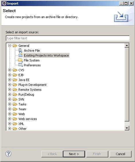
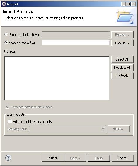
Open Eclipse by going to Programming and Scripting | Eclipse IDE for Java Developers | Helios. Import the jar file into your Eclipse workspace by going to File | Import... then selecting General | Existing Projects into workspace then selecting Select archive file:, browsing to where you downloaded the jar file and clicking Finish.
To compile and run the assembler, in Eclipse, open Asm.java and create a new run configuration by going to Run | Run Configurations..., selecting Java Application and clicking the new icon in the top left. Then select the Arguments tab and enter add.asm and click Run. There should now be two more files in the current directory add.mif and add.rmb. These files are both the assembled program but in different formats. Quartus accepts the Memory Initialisation File (mif) format and Modelsim accepts the $readmemb (rmb) format.
Simulating an existing program
In Quartus, go to Assignments | Setting | EDA Tool Settings | Simulation. Here, under Tool name select ModelSim-Altera. Then press Apply and OK to finish.
Next, start Modelsim from Quartus via Tools | Run EDA Simulation Tool | EDA RTL Simulation.
Driving Modelsim using a "do" script
As well having a graphical interface, Modelsim also has a scriptable command interface. Commands can either be typed line by line at the prompts Modelsim> and VSIM N> or saved to a ".do" script and run. We've provided you with ttcsim.do which will simulate the TTC running the add.rmb machine code that the assembler created.
Just type do ttcsim.do into the Modelsim command prompt. It is possible that you'll need to cd into your project directory first.
Modelsim will then simulate the design as if the circuit had been running for up to 30ns (since we tell it to "run 30ns" in the "do" script) or until a $stop in the SystemVerilog is reached. Waveform traces will be produced which can be useful to debug the processor, though you will probably find that you do not need to look at these. The simulation also produces an instruction execution trace (via $display statements in the SystemVerilog) together with output results.
Tip: the ttcsim.do script contains the line:
vsim -Gprogpath_rmb=add.rmb -Gdebug_trace=1 TestTinyComp
TestTinyComp refers to the SystemVerilog module inside ttc.sv which will provide test input stimulus. Change add.rmb to change which machine code is loaded before the simulation starts. Change -Gdebug_trace=1 to -Gdebug_trace=0 if you just want to see the results output without an instruction trace.
Driving Modelsim using the GUI
An alternative to using the ttcsim.do script is to invoke the simulation using the GUI. In Modelsim we first need to compile ttc.sv by going to Compile | Compile, finding ttc.sv, selecting it and clicking compile. Next, we will start simulation. Go to Simulate | Start Simulation, expand work and select TestTinyComp. Next, in the Others tab, click Add... in the Generics/Parameters part. As the name put progpath_rmb. As the value put the absolute path to add.rmb. Finally, click OK to begin the simulation.
Add waveforms
To add waveforms to the wave window, right click a signal, Add | To Wave | Selected Signals. To add all the signals in the design, right click any signal, Add | To Wave | Signals in Design. This won't include signals with more than one dimension, such as memories. Add all the signals then manually add the register file TestTinyComp/dut/rf_block. In this simulated version of the TTC there is no data memory, just a ROM, a register file, an input port and an output port.
To run the program for 100ps go to Simulate | Run | Run 100. The simulator is currently set up so 1ps is the smallest unit of time. TestTinyComp is written such that 1 clock cycle = 10ps. So running for 100ps is the same as 10 clock cycles or 5 non-data-memory instructions. Run the program until you're happy you can see it performing an add and then stalling when it runs out of input parameters.
Task: writing an assembly program to do an unsigned multiply of two numbers on the input port
You may have noticed this processor has no multiply function. In the second lab we will add one since we will be plotting the Mandelbrot set, a task requiring much multiplication but for the time being we will implement one in software. By the end of this section you will have produced an assembly program to read two integers from the input port, multiply them and output the result. The inputs are 32-bits and just a 32-bit result is required.
There are many ways to multiply two integers in software. The most obvious is probably simply repeated addition. That is to say, add an input a to an accumulator and output c an input b times. After this procedure c=a*b if b is non-negative. This takes time O(2^n) for a machine with word size n with constant time addition since the worst case is having a large b and having to add b times. The largest b=2^n-1.
Instead, binary long multiplication, aka "shift and add" can be used. Here's an example multiplying 7*11.
     0111
    *1011
     ----
      111
     1110
   111000
   ------
  1001101
= 77 as required. This is O(n) since addition is treated as constant time and the number of additions is the number of set bits in b, the worst case is b has all the bits set.
In Eclipse, open ShiftMult.java which is an implementation of this for Java. The function mult operates only on signed 32 bit integers (although it is actually doing unsigned multiplication) and so corresponds fairly closely to the assembly code you will write.
In Eclipse, create a new file named mult.asm and write assembly code which will read two integers from the input port, multiply them and then output the lower word of the result on the output port. Remember, reading a word from the input port to r1 would be achieved using r1 <-in, writing using r0 r1 ->out where r1 in this example contains the value to be output and r0 is the unused desitnation register (a scratch register). To assemble it you will need to change the argument of Asm.java to mult.asm under its run configuration. Create a new simulation "do" script (e.g. "ttcsim_mul.do") and simulate you machine code. Modify the TestTinyComp module in ttc.sv so that the following multiplications are tested: (3*1), (3*10000), (13*19), (13*0).
A successful demonstration of your program multiplying the numbers is the ticking criteria.