ECAD and Architecture Practical Classes

Exercise 2 (optional): Verilog simulation

Part A: Introduction to simulation in Modelsim

Fully implementing a system is very expensive, taking both time (FPGA: minutes/hours, ASIC: months/years) and money (ASIC: millions of dollars). Making a mistake - a system that does not function as intended - can thus be very costly. The later a bug is found, the more expensive it is to fix.

To reduce risk and save time and money, a key part of the design process is verification: ensuring correctness of the system. We wish to discover bugs as rapidly and cheaply as possible.

In these labs we'll apply a similar approach - verifying in simulation allows rapid development without having to wait for long FPGA build times.

Hardware/software systems are also very complicated, and so simulating a chip with billions of transistors at the level of basic physics would be intractable. For this reason we break down the design into pieces and simulate at the highest layer of abstraction sufficient to test the required properties. Abstractions are used to reduce overall complexity, and implementations can be tested against their abstractions.

Behavioural simulation: simulates the behaviour of a component without considering its implementation. For example, we can test a logic function obeys q=x+y without considering how it might be implemented in terms of half adders or NAND gates. In a behavioural simulation, it is possible to describe systems that may have no physical implementation, such as an infinite-length counter which never overflows.
Functional simulation: considers a particular implementation of the system, for example the circuit described in terms of logic gates, standard cells, transistors or silicon layout. As we go down the design process we can confirm that one level behaves the same as the previous level - for instance that a given transistor circuit does implement q=x+y within acceptable parameters.

When writing SystemVerilog, it is common to also write test harnesses to test the resultant hardware behaves correctly. These can make use of a number of non-synthesisable constructs. We'll introduce some of these to you here since they are used in the labs.

Four-valued logic

Signals can be other than high or low:

Value	Meaning
0	False
1	True
x	Undefined
z	High impedance

x appears in simulation for an uninitialised state - for example a register with unknown contents. Undefined values propagate: a combinational function f(a,b,c) returns x if any a, b or c are x. x has no physical realisation: the implementation will choose 0 or 1 (not always consistently).

z represents tristate, the third physical state of a wire, when we force neither a high or low voltage on it but instead disconnect it. Most commonly it is used for bidirectional pins, where we receive by tristating (not driving) the pin and listening if some other component is driving the pin high or low. Tristates are rarely used within a chip, but off-chip the I2C interface is an example of this usage.

Modelling delays

A simulation often wants to implement a fixed delay as part of a testbench, for example a delay of 5 nanoseconds.

`timescale 1ns / 1ps

module delay5ns (input logic in_signal, output logic delayed_signal);
  assign #5 delayed_signal = in_signal;
endmodule

The timescale indicates we use units of 1 nanosecond, but with a resolution of 1 picosecond. In other words, if we wrote a time of 1.2345 it would be rounded to 1.235ns.

A delay like this has no physical meaning, but is often used to generate a clock in testbenches, for example to generate a 50MHz clock (10ns per half-cycle):

  always #10
    clk <= !clk;

When a design has a candidate implemention on a target platform (FPGA, ASIC) we might perform timing extraction which measures the gate and wire delays of the circuit as implemented. The process of back annotation then allows adjustment of these delays in the structural SystemVerilog to match the realised circuit, and we can then re-run our tests to check for correctness.

Event-driven simulation

A naive simulation would be to recalculate the state of all logic signals every time step. In the above code, we set a time resolution of 1 picosecond, i.e. 10^-12 seconds. The naive simulator would thus perform 1 trillion iterations per second of simulated time - this would be very slow on a modern computer. Most of that would be inefficiently simulating logic states which are constant.

Instead event-driven simulation only simulates changes. Each gate is an object (with internal state). Signal or state changes are events with timestamps. Every object receives events and can decide to generate other events with a timestamp in the future, which are placed in a queue.

The simulator iterates over the event queue, picking the oldest event and passing to the appropriate object. If the output of that gate changes, an event with a new value and a future timestamp is placed in the queue. In this way, components which are idle take no simulation time.

The output of such a simulation is a list of (signal,timestamp) pairs of changes. These can be represented as a waveform - for instance in a Value-Change-Dump (.vcd) file - or on screen.

SystemVerilog system tasks

Additionally, simulations can have other statements such as:

$display("Value of foo = %d", foo); // print some text to the log (format string syntax as C/C++).

$display("Time is %t", $time); // print the simulation time.

$dumpfile("example.vcd"); $dumpvar; // dump all variables to a named .vcd file

$finish; // end the simulation

Exercise 2a: Prepare to simulate your traffic light controller

In the last but one web tutor exercise, you designed a traffic light controller. In preparation for the tickable exercises, let's have a go at simulating your design using the ModelSim simulator you'll be using for the ticks. We're going to use this tool on an MCS Linux machine or within the course virtual machine.

First create a directory exercise0 for your simulation project and copy in your SystemVerilog code for your tlight module (including the header and footer). Put this into a file of the same name as the module with suffix .sv (for SystemVerilog), i.e. tlight.sv.

Before we can simulate the design, we will need a test bench to provide input stimulus. In this instance there is just one input, the clock. We can provide a clock as follows and instantiate the tlight module to test it. Let's create a tb_tlight.sv in which we will call the test bench tb_tlight and the instance of tlight to test dut (Design Under Test), viz:

`timescale 1ns / 1ps

module tb_tlight(
  output r,
  output a,
  output g);

  logic clk;      // clock signal we are going to generate

                  // instantiate design under test (dut)
  tlight dut(.clk(clk), .r(r), .a(a), .g(g));

  initial         // sequence of events to simulate
    begin
      clk = 0;   // at time=0 set clock to zero
    end

  always #5       // every five simulation units...
    clk <= !clk;  // ...invert the clock

                  // produce debug output on the negative edge of the clock
  always @(negedge clk)
    $display("time=%05d: (r,a,g) = (%1d,%1d,%1d)",
      $time,      // simulator time
      r, a, g);   // outputs to display: red, amber, green

endmodule // tb_tlight

Step 3: Simulate your design

To start up ModelSim, we first need to setup paths and environment variables to use the ECAD tools, depending on your setup. Open a new terminal window. On the MCS you will need to source the appropriate setup.bash script as described in the setup instructions.

To start the ModelSim simulator, type:

vsim

This will open up a graphical window similar to the following:

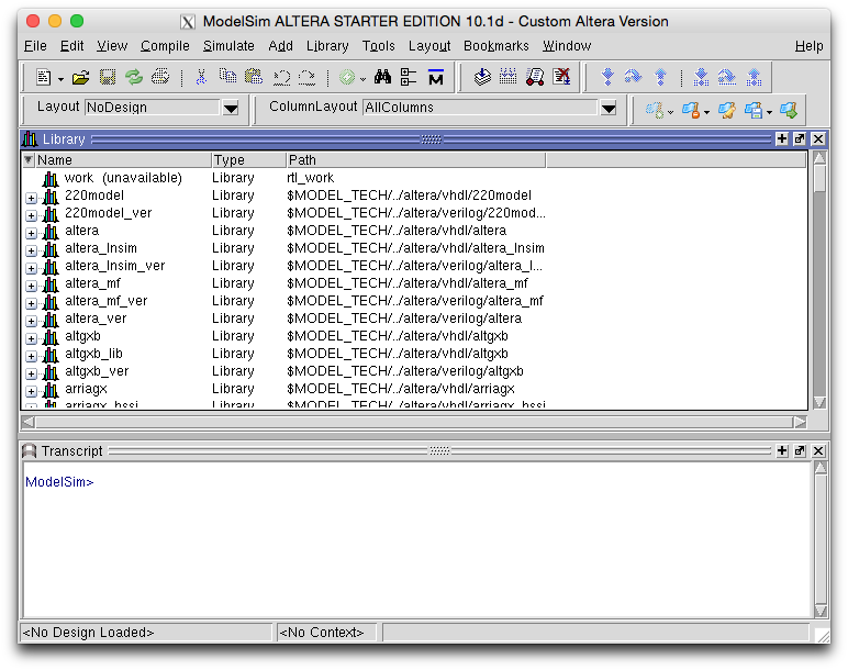
The main ModelSim window consists of three areas. The "Transcript" area contains a command line terminal that you can use to give commands. All functions in ModelSim are accessible through the menus, but the command line can help in scripting up various sequences of operations that you wish to repeat. In addition, the Transcript area will show the output of any print statement that has been added to your component design.

On the left there is the library panel. This panel contains various libraries that contain one or more (compiled) components. To create a new library, click File->New->Library. ModelSim mandates that you create a library called "work" (Library Name and Library Physical Name), in which all custom compiled projects are stored. (If you already have a library 'work (unavailable)', right click it, go to New->Library and 'Create: a new library' with physical name 'work').

To compile your design in ModelSim, click on Compile->Compile.... From the file chooser dialogue, you can now navigate to the folder where you stored your sources. Double-click on the files that you wish to compile (tlight.sv and tb_tlight.sv). When unsuccessful, the transcript area should give you some hints about why it failed to compile. For more info, you can also look in the compile summary, that can be opened by clicking Compile->Compile Summary. ModelSim is only able to figure out dependencies on other modules after they have been compiled, so either select all components by holding ctrl and click on all source files, or compile your components from the bottom up.

If everything went well, your components should now have appeared in the library "work" (you may need to click the + symbol by work to see the compiled modules). By double-clicking on the top-level component (tb_tlight), you will start a simulation. This will add the simulate buttons to the toolbar area above and insert another area in the ModelSim GUI called objects that contains all signals of the module selected in the "Sim" area, defaulting to the top level module.

There should be a "Wave" panel which contains no signals (if not click "View" and then "Wave" to show it). Add the signals r, a, g and clk from the "Objects" panel by dragging them to the "Wave" panel.

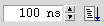
Now to simulate the design. Look for the simulation time period (typically 100ns) and the "Run" button to the right of it which looks like:

You might wish to press the zoom-in button a couple of times to get a simulation like the following.

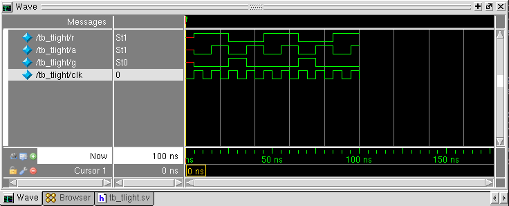
In the "Transcripts" window you should also see the output from the $display statement in the test bench which should produce the following which provides the same information as the waveform output:

# time=    0: (r,a,g) = (x,x,x)
# time=   10: (r,a,g) = (1,0,0)
# time=   20: (r,a,g) = (1,1,0)
# time=   30: (r,a,g) = (0,0,1)
# time=   40: (r,a,g) = (0,1,0)
# time=   50: (r,a,g) = (1,0,0)
# time=   60: (r,a,g) = (1,1,0)
# time=   70: (r,a,g) = (0,0,1)
# time=   80: (r,a,g) = (0,1,0)
# time=   90: (r,a,g) = (1,0,0)
# time=  100: (r,a,g) = (1,1,0)

See the hints if your simulation produces x's as output.

Step 4: Script the simulation

During test driven hardware development, simulation runs are frequent and using the GUI to setup the simulation run each time is a bit tedious. The solution is scripting. ECAD tool vendors often use the TCL scripting language. Here is an example commented "do" script in TCL.

# set up the "work" library
vlib work
# compile our SystemVerilog files
vlog tlight.sv
vlog tb_tlight.sv
# point the simulator at the compiled design
vsim work.tb_tlight
# add waveforms to the "Wave" pane
add wave -position insertpoint \
  /tb_tlight/r                 \
  /tb_tlight/a                 \
  /tb_tlight/g                 \
  /tb_tlight/clk
# run simulation for 200 nanoseconds
run 200 ns

If you copy the above script into a file runsim.do and change ModelSim's working directory to match (the "Transcript" pane has a cd command), you can execute it by typing the following into the "Transcript" pane of ModelSim:

do runsim.do

You can also run ModelSim (vsim) from the command-line only with no GUI. This can be useful when you just want the output from $display statements and no waveform viewer. For example:

vsim -c -do runsim.do

Adding "quit" to the end of the runsim.do script will cause vsim to cleanly exit after the simulation run. The "add wave ..." statement is redundant if there is no waveform window, so can be removed.

Resources

There is a ModelSim quick reference guide on the downloads page.

Optional exercise

Try out your electronic dice in ModelSim. You will need to provide a "button" input. One approach is to extend the initial block with changes of state to a "button" register using specified delays and non-blocking assignment, viz:

initial
  begin
    clk = 0;
    button = 0;
    // after 20 simulation units (2 clock cycles given the clk configuration)
    #20 button = 1;
    // after 100 simulation units
    #100 button = 0;
  end

Hints and Tips

You may find that your simulation produces x's as output due to registers being uninitialised at the start of the simulation. For FPGA designs we're sometimes lazy and rely on the FPGA to come up with registers reset to zero. This can be mimicked in simulation by adding an initial statement, e.g. for tlight you might add:

initial state=0;

When you change a file, you'll need to recompile it and restart simulation so that your changes take effect.

Initial statements are ignored when synthesising a design into a real circuit. Also note that this might not work if you assign to state elsewhere in an always_ff block, since the tools might not allow logic to be driven from two different blocks. A synthesisable (i.e. better) approach to initialising state is to use reset signals. For example, for tlight you might add another input called "rst" and for the always_ff block add:

always_ff @(posedge clk or posedge rst)
  if(rst)
    state <= 3'b000;
  else
    ...

In your test bench you'd need to add the rst signal as a register and initialise it for simulation viz:

  initial          // sequence of events to simulate
    begin
      clk = 0;     // at time=0 set clock to zero and reset to active (1)
      rst = 1;
      #20 rst = 0; // after 2 clock ticks set reset to inactive (0)
    end

SystemVerilog is not a type-safe language, which means it will silently convert values of different types. One of the most annoying features for debugging is it will create undeclared signals (`implicit nets') for you if you don't define them. This can be problematic if you mistype a net name, because the correct version and the typo version will not be connected together, and the tools may synthesise these away. You can force an error to be generated with:

  `default_nettype none

in your source file. However this does not work for all compilation tools.

Part B: Human Input in simulation

Introduction

We have combined a DE1-SoC board from Terasic with our own input/output board mounted on the back. Output is in the form of an LCD and some tri-colour LEDs. For this exercise we will focus on the inputs: rotary dials and switches.

Rotary Dials

Rotary encoders are widely used for human input from old mechanical mice to the rotary knob you find on a Nest thermostat. There are also many industrial applications: see Wikipedia on rotary encoders for details.

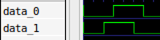
The two rotary dials on the DE1-SoC I/O board are incremental rotary encoders which have mechanical contacts. There are two outputs which produce a Gray code sequence when they are turned. A full rotation is 24 discrete steps. For a clock-wise step, a clean signal will have a waveform as follows:

For a counter-clock-wise step, the waveform looks as follows:

The output signal is digital and asynchronous; the time between two edges on a waveform is only determined by the physical action of turning the knob. Physically this is implemented by moving a conductive part over a two-channel "code track" on a disc. Wiggle in the conductive part causes a bouncy output signal from the rotary encoder. In practice, this means that if you measure the signal produced by a clock-wise turn, the result will look more fuzzy. By using an oscilloscope, we measure the following: `

Although we can definitely recognise the square wave of a counter-clock-wise turn in this diagram, the noise we observe could make it difficult to make decisions in a digital system. In two places, a high signal drops to low for periods as much as 0.2ms. To turn this signal into a clean square wave that we can interpret in some control logic, we must first apply some filtering known as debouncing.

Synchronising external inputs

First, before we can pass signals into our logic, we need to synchronise them with our clock. If the input to a flip-flop changes during its setup and hold periods, there is a chance the flip-flop will go metastable - produce an output voltage that's somewhere between 0 or 1. If we provide this signal to another logic gate, that may also go metastable, and so on through the system, leaving the system in an indeterminate state.

The probability of metastability decays exponentially with time. Hence a common design pattern is the two-flop synchroniser:

By delaying the signal for a least a whole clock period, we give time for the metastability to decay to a stable value, substantially reducing the probability the output of the second flip-flop is metastable.

Such a synchroniser is also common for clock-crossing: when signals synchronous to one clock are converted to being synchronous to another.

Exercise 2b: Debouncer

Implement debouncing logic in SystemVerilog. It will take the following input signals:

A clock signal
A bouncy signal

The output of this component is a debounced (i.e. cleaned up) signal

Assume that this logic block receives an input clock of 50MHz. Your logic should sample the input line and change the value of its output line only if a signal has been in the same state for a certain amount of samples. Choose this time interval such that it is long enough to detect the spikes as seen in the measurement above, but short enough to still be able to determine which of the two lines was set to high first.

Ensure you synchronise each asynchronous input using a two-flop synchroniser as depicted above. You may find it useful to make a separate synchroniser module.

We encourage you to do test driven development using the simulation techniques you have already learnt. To help you get started, we've created a simple test bench tb_debounce.sv and a suitable "do" script tb_debounce.do.

Navigate to the ecad_labs/ex2_rotarysim directory. It contains template "debounce.sv" and "rotary.sv" files along with some test bench files.

When implementing this component in SystemVerilog, please store the file as "debounce.sv" and use the following template so that it matches up with the test bench.

module debounce
  (
        input wire       clk,       // 50MHz clock input
        input wire       rst,       // reset input (positive)
        input wire       bouncy_in, // bouncy asynchronous input
        output reg       clean_out  // clean debounced output
   );

        /* Add wire and register definitions */

        /* Add synchronous debouncing logic */

endmodule

Tips:

First, consider how to detect a change in the input line from one clock period to the next.
Then use a counter to reflect that change on the output only after a sufficient number of clock cycles have elapsed.
Until that period has elapsed, ignore all further changes on the input line.

Exercise 2c: Rotary Decoder

Create a new SystemVerilog module that implements control logic for interpreting the output of the rotary encoder. The input of your control logic will take three signals:

A 50MHz clock signal.
A reset signal (active-high, meaning that reset is asserted when its signal is 1).
A two-bit rotation signal.

Its output will be:

An rotary_pos 8-bits integer value representing the position of the knob relative to its begin position.
A rot_cw signal asserted for one cycle when a clock-wise rotation is detected.
A rot_ccw signal asserted for one cycle when a counter-clock-wise rotation is detected.

Your logic is expected to perform the following:

Debounce the input signals.
For every clock-wise detected step, increment the output value by one and assert the rot_cw signal for one cycle.
For every counter-clock-wise detected step, decrement the output value by one and assert the rot_ccw signal for one cycle.
When the reset signal is asserted, reset the counter to 0.

When implementing this component in SystemVerilog, please store the file as "rotary.sv" and use the following template.

module rotary
  (
        input  wire clk,
        input  wire rst,
        input  wire [1:0] rotary_in,
        output logic [7:0] rotary_pos,
        output logic rot_cw,
        output logic rot_ccw
   );

        /* Add wire and register definitions */

        /* Instantiate debouncing components */

        /* Synchronous output value manipulation logic */
        
 endmodule

Test your module using tb_rotary.sv and tb_rotary.do supplied.