
Course pages 2013–14
Experimental Methods
An introduction to data analysis using R
R is a free suite of software for statistical computing that runs on Windows, Unix and MacOS.
Download a copy of R from the Comprehensive R Archive Network (CRAN).
See Peter Dalgaard's book or the Data Analytics web site for details of R, or just type
?routine
for on-line help about a particular function.
Preliminaries
Examples of different techniques will be illustrated with some data from Chapter 4 of Lazar (Table 4.11). It could be entered in a text file, lazar.txt, laid out with tabs as follows:
std	prd	spc
245	246	178
236	213	289
321	265	222
212	189	189
267	201	245
334	197	311
287	289	267
259	224	197
This would be read into R as follows:
times <- read.table ("lazar.txt", header=T)
attach (times)
giving three vectors std, prd and spc.
Warning: The same set of data will be analysed here as if it has been collected in several different ways. Any real data could only be analysed in ways that were appropriate for the design of the experiment.
Visual inspection
Inspect the data by grouping it into bins and plotting the resulting histogram:
bins <- seq (175, 350, 25)
hist (std, breaks=bins)
Check for normality
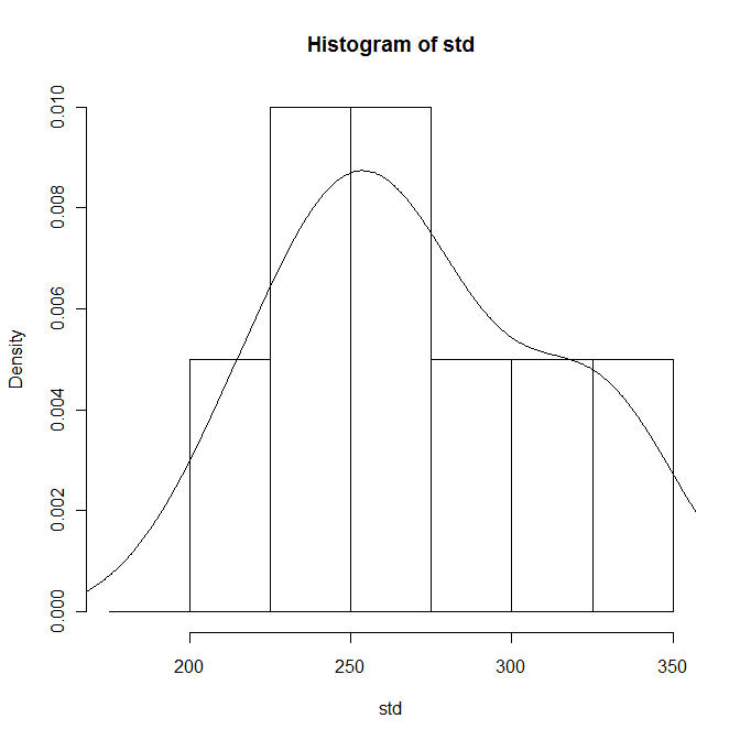
Most of the statistical tests rely on the sample data, or at least the residuals, having a normal distribution. This can be checked visually by superimposing a continuous distribution curve over the histogram. The histograms should be scaled as probabilities first:
hist (std, breaks=bins, prob=T)
lines (density (std))
Alternatively, compare quantiles in the sample data with quantiles in a normal distribution with the same mean and standard deviation, and then superimposing a line at 45°:
qqnorm (std)
qqline (std)
Investigating relationships
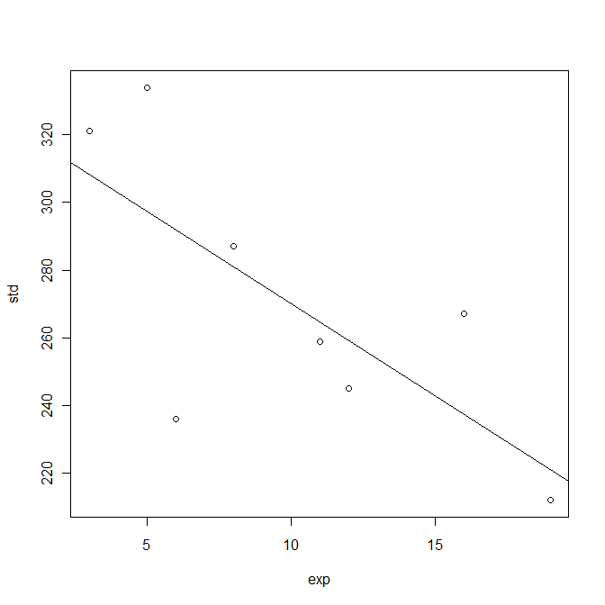
Each participant's number of years' experience using computers from Lazar Table 4.20 could be stored in a vector, and then the correlation with the standard data entry time investigated as follows:
exp <- c (12, 6, 3, 19, 16, 5, 8, 11)
plot (exp, std)
m <- lm (std~exp)
coef (m)
abline (m)
summary (m)
Observe that the slope of the least-squares line (the regression coefficient) is negative, and that the squared Pearson correlation coefficient R2 is 0.5222, giving a p-value of 0.04286 which is significant at the 95% level.
The actual residuals are available as:
resid(m)
and it would be worth inspecting their distribution.
Box plots
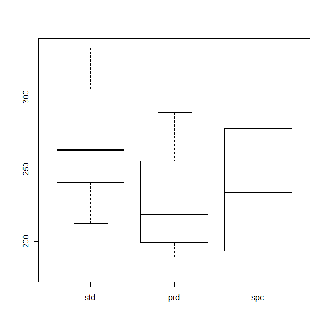
The distributions can be compared using box plots:
alltimes <- c (std, prd, spc)
method <- gl (3, 8, 24, labels = names(times))
plot (method, alltimes)
The horizontal bars in the middle of the boxes indicate the median value, and the boxes themselves approximately cover the central two quartiles.
Mean and standard deviation
The means and standard deviations of the three series can be calculated:
tapply (alltimes, method, mean)
tapply (alltimes, method, sd)
t test
The graphs and box plots suggest that the task completion time for predictive entry is less than for standard entry. This can be checked with a t test:
t.test (std, prd, alternative="greater")
Observe that t is 2.1688 and p-value is 0.02414. This would be reported as:
An independent-samples t test showed a significant effect of the predictive software against the standard input on the task completion time (t(13.7) = 2.17, p < 0.05).
If the data had been collected in a paired-samples experiment, the analysis would be:
t.test (std, prd, alternative="greater", paired=T)
In this case, t is 2.6313 and p-value is 0.01693. This would be reported as:
A paired-samples t test showed a significant effect of the predictive software against the standard input on the task completion time (t(7) = 2.60, p < 0.05).
The graphs also suggest that there is little difference between predictive and speech-based entry. A t test shows that t is -0.4325 and p-value is 0.3363. This would be reported as:
An independent-samples t test showed no significant difference between the speech and predictive software on the task completion time (t(12.8) = 0.432, p > 0.05).
One-way ANOVA
Analysis of variance compares the means of two or more groups. (If there are only two groups, this is the same as a t test.)
a <- aov (alltimes~method)
summary (a)
Observe that F value is 2.1738 and Pr(>F) is 0.1387. This would be reported as:
A one-way ANOVA test showed no significant effect of the three input methods on the task completion time (F(2,21) = 2.17, p > 0.05).
Repeated measures ANOVA
The one-way ANOVA assumes a between-group design which involves recruiting 24 participants. A within-group design is more economical, inviting each participant to undertake all the tasks (as shown in Table 4.11 of Lazar). This requires a further factor in the analysis:
participant <- gl (8, 1, 24)
a <- aov(alltimes~(method+Error(participant/method)))
summary (a)
Pr(>F) is 0.0868, outside the 95% confidence level. This would be reported as:
A repeated measures ANOVA test showed no significant effect of the task on completion time (F(2,14) = 2.93, p > 0.05).
Factorial ANOVA
Suppose that trials of the three input methods were also performed for a second task, giving the data in Table 4.9 of Lazar. alltimes now contains 48 values and the corresponding factors and analysis are:
method <- gl (3, 16, 48, labels = names (times))
task <- gl (2, 8, 48, labels = c ("Transcription", "Composition"))
a <- aov (alltimes~task*method)
summary (a)
Observe that the additional data reveals a difference between the different methods but not between the tasks. This would be reported as:
A factorial ANOVA test showed no significant effect of the task on completion time (F(1,42) = 1.41, p > 0.05). There was a significant effect of input method on the completion time (F(2,42) = 4.51, p < 0.05).
The same data could be analysed as a repeated measures experiment (as shown in Table 4.14 of Lazar) by introducing a further factor:
participant <- gl (8, 1, 48)
a <- aov(alltimes~(task*method+Error(participant/(task*method))))
summary (a)
The task type has a significant effect on the time taken to complete the task, but there is no significant difference between the input methods and no interaction effects between the task and input method. This would be reported as:
A repeated measures ANOVA test showed a significant effect of the task on completion time (F(1,7) = 14.2, p < 0.01). There was no significant effect of input method on the completion time (F(2,14) = 2.93, p > 0.05), and there was no interaction effect between the independent variables (F(2,14) = 0.760, n.s.).
Mixed design ANOVA
A within-group design requires each participant to undertake all the tasks, which may be tiring. A mixed design (split-plot) has some particpants undertaking only some of the tasks (as shown in Table 4.17 of Lazar). This requries slighlty different factors in the analysis:
participant <- gl (16, 1, 48)
a <- aov(alltimes~(task*method+Error(participant/(task*method))))
summary (a)
There is no significant difference between the participants who undertook the two tasks, but there is a significant difference between the three input methods. There are no interaction effects between the task and input method. This would be reported as:
A split-plot ANOVA test showed a significant effect of the input method on the completion time (F(2,28) = 5.70, p < 0.01). There was no significant difference between the participants undertaking the two tasks (F(1,14) = 0.995, n.s.) and there was no interaction effect between the independent variables (F(2,28) = 0.0373, p > 0.1).
Further examples
See the Personality Project web pages for further examples.
Google has published a style guide for programming in R. The is also an R client for the Google Prediction API.
The formulae for models in R are described in Symbolic description of factorial models for analysis of variance by GN Wilkinson and CE Rogers (Journal of the Royal Statistical Society 22(3), 1973, pp. 392-399).