
Course pages 2013–14
Experimental Methods
Investigating experimental data
The first step is to inspect the data visually:
- Use histograms to investigate possible distributions. In particular, check that residuals are approximately normally distributed.
- Use box plots to investigate the likely significance of differences between factors.
- Use scatter plots to investigate relationships.
Then more powerful analyses based on probability can be used to estimate the significance of results.
Software
There are many special-purpose packages for statistical analysis, notably R (which is available as a free download for Windows, Unix and MacOS) and SPSS (which is available on PWF computers). Many simple analyses can also be undertaken using Microsoft Excel.
The University Computing Service runs a couple of useful self-service training courses on statistics and SPSS:
Both are available directly on PWF systems.
There are further pages in this section on data analysis in Excel and data analysis in R.
More technical questions can be taken to the University's Statistics Clinic.
Tabletop collaboration
The following description covers the preparation, initial investigation and statistical analysis of an experiment to study collaboration using a tabletop display. Pairs of participants undertook a task using tabletop displays in three different ways: sitting side-by-side at the same display, sitting logically side-by-side but at separate displays that were showing the same data, and sitting centrally at separate displays.
Read the paper on Territorial coordination and workspace awareness in remote tabletop collaboration for full details.
Preparation
The dependent variable for the study was the partitioning index measuring the extent to which participants worked only on one side of the table while collaborating. A pilot study suggested that the index was about 0.4 for co-located collaborators, but about 0.2 for remote collaborators independently of where they sat. Both measures had a standard deviation of about 0.15.
A power calculation was performed to calculate the number of pairs of participants that would be required for a power of 0.8 and a significance level of 0.05:
n ≈ 16 × s2 ÷ δ2 = 16 × 0.152 ÷ 0.22 = 9
So 18 participants were recruited and divided into 9 pairs. A repeated measures design was used, with the order of trying the three methods counterbalanced using a Latin square.
Preliminary investigation
The data were collected and tabulated in a spreadsheet:
| A | B | C | |
|---|---|---|---|
| 1 | Pair | Code | Index |
| 2 | 1 | CA | 0.387 |
| 3 | 1 | RO | 0.206 |
| 4 | 1 | RA | 0.271 |
| 5 | 2 | CA | 0.678 |
| 6 | ... | ... | ... |
This was saved as comma separated values in the file collaboration.csv and read into R:
data <- read.csv("collaboration.csv")
attach(data)
Inspect the data:
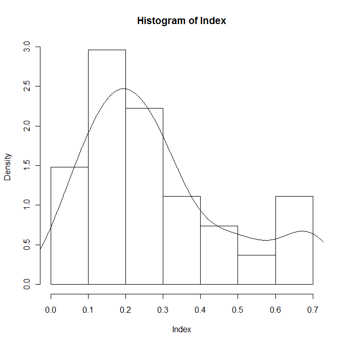
hist(Index,prob=T)
lines(density(Index))
The distribution of the index looks bimodal, as anticipated, so separate the three conditions and inspect them individually:
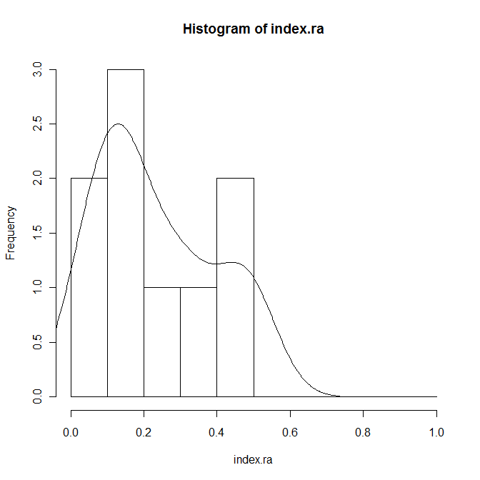
index.ra <- Index[Code=="RA"]
hist(index.ra,prob=T,breaks=seq(0,1,0.1))
lines(density(index.ra))
Check for normality:
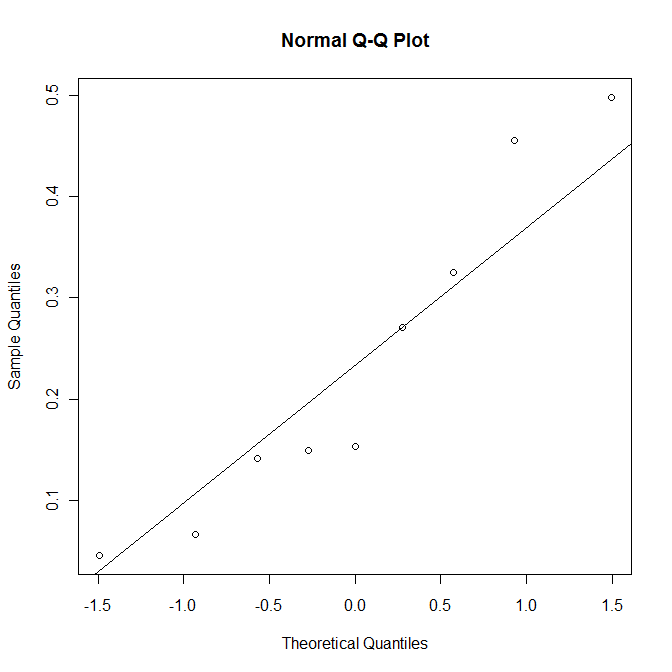
qqnorm(index.ra)
qqline(index.ra)
shapiro.test(index.ra)
The p-value of 0.29 is sufficiently large not to reject the null hypothesis. In other words, it is plausible to treat the data as normally distributed.
Check the remote overlaid and co-located adjacent distributions in the same way.
Calculate means and standard deviations:
tapply(Index,Code,mean)
tapply(Index,Code,sd)
The mean co-located index is 0.44 and the mean remote index is 0.21, and average standard deviation of the indices is 0.16. Check the power:
power.t.test(n=9,delta=0.23,sd=0.16,sig.level=0.05)
This suggests that there is an 82% chance of detecting a true effect.
Compare the three conditions visually:
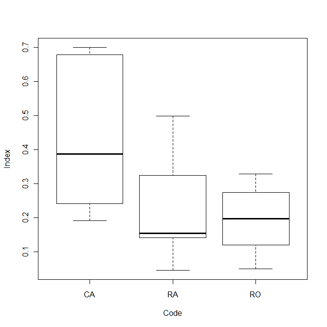
plot(Index~Code)
Statistical analysis
Perform a one-way repeated measures analysis of variation:
summary(aov(Index~(Code+Error(Pair/Code))))
There is a significant effect, F(2,16) = 7.02, p < 0.01.
Perform pairwise t-tests:
t.test(index.ca,index.ra,paired=T)
t.test(index.ca,index.ro,paired=T)
t.test(index.ra,index.ro,paired=T)
There is a significant difference between CA and RA, t(8) = 3.64, p < 0.01, and between CA and RO, t(8) = 2.83, p = 0.022. There was no significant difference between RA and RO, t(8) = 0.683, n.s.
Strictly speaking, the alterative form should be used to correct for multiple testing:
summary(aov(Index~(Code+Error(Pair/Code))))
This identifies the same differences.
Comparing different pairs of participants
Compare remote partitioning index with co-located one:
plot (index.ca,index.ra)
m <- lm (index.ra~index.ca)
abline (m)
segments (index.ca,fitted(m),index.ca,index.ra)
summary (m)
About 36% of the variance in the remote index can be explained by the participants' co-located index. The probability of achieving this good a fit by chance is just over 0.05, which is too high to be significant.