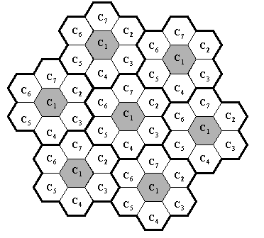
2.1.1          Distributed Non-Measurement (DN)

In the Distributed Non-measurement  quadrant the base station does not have access to the current interference environment information.  Therefore, a priori knowledge of the system and network are required to assigned channels to calls.  The information required may be the location of the base stations, an estimate of the offered traffic, the propagation model of the coverage area and the number of available channels.  FCA belongs to this quadrant since it relies heavily on a priori information and does not require up to date interference information during system operation.  However, the channels do not change during system operation and hence the initial channel assignment is important.  Another method falling into this category is the random channel allocation (RND).  The methods surveyed in this section have primarily been designed with voice services in mind.

2.1.1.1       Random Channel Allocation

Given a list of available channels, Random Channel Allocation (RND) [11], [56], [50] selects a channel randomly based on a uniform distribution.  The idea is similar to Frequency Hopping, where the channels are picked at random and are usually changed at random during a call.  For example, if there are five channels where one is bad, the call will only spend a short time in a bad channel and hence averaging out the interference among all channels.  This is effective if the number of available channels is large and is very simple to implement and does not require a lot of prior planning in the network.  Averaging interference has a poorer performance compared to an algorithm that avoids interference [12].  RND is usually used as the lower bound performance for channel allocation methods.  This is because the RND algorithm does not use any current or prior information to allocate a channel.

2.1.1.2       Fixed Channel Allocation

Consider a cellular network with uniform traffic (i.e. each cell is the same size and has the same amount of offered traffic) and the layout shown in Figure 2.1.  If the required SIR is 17 dB and the cell radius is fixed at R_b, for a given propagation model the reuse distance  R_u and cluster  size N_c can be found.  In FCA, the set of channels C is usually divided into channel groups [1].  If N_c = 7, each cell in the cluster will take one of the channel groups, i.e., the channels are divided into 7 groups C = {C₁, C₂, C₃, C₄, C₅, C₆, C₇}, where C_j is a distinct set of channels.  Using this a priori information, the channels can be allocated with the reuse pattern shown in Figure 2.3.

Figure 2.3: Channel Allocation in a network with uniform traffic distribution.

It is common for a network to have non-uniform traffic.  For example, a cluster of cells may cover a busy shopping area (heavy traffic) and a neighbouring cluster of cells may cover a residential area (low traffic).  If the reuse pattern shown in Figure 2.3 is applied to this situation, the channels may not be utilized efficiently.  For example, the cells with heavy traffic may not have enough channels to ensure a low blocking probability while the cells with low traffic may not use all the channels assigned to them. 

For a fixed number of channels, a smaller reuse ratio  gives higher capacity.  This is because a smaller reuse ratio leads to a smaller cluster size and therefore the same number of channels is distributed to a smaller number of cells.  The reuse pattern may also differ if the cell radii are not constant.  Hence, the uniform reuse pattern in Figure 2.3 may not be applicable in these cases.

In a cellular network with non-uniform traffic, the compatibility matrix is used as part of the a priori information.  The frequency separation between two base stations depends on the level of interference that would give an acceptable SIR.  If two base stations are a sufficient distance apart such that the co-channel interference is acceptable, the frequency separation between these two base stations is zero.  By estimating the frequency separation between every base stations the compatibility matrix is formed.

The optimum solution (i.e. one that uses the least number of channels) to a channel allocation problem is difficult to obtain particularly for a large network.  Although finding the optimum solution is possible (e.g. using brute force), it may not be practical.  It is desirable to have a solution that is as close as possible to the optimum solution and there are a large number of publications devoted to achieving this aim, some of which are highlighted later in this section.  The theoretical lower bound solution  C_L (C_MIN ³ C_L) is proportional the product of the highest traffic demand d_j* and the channel separation c_j*,j* at base station j* thus [22]:

Where it is assumed that c_j,j > c_j,k for all k and usually c_j,j = c_k,k for j ¹ k.  For a solution that uses C channels, it is desirable that the channel numbers are as close together as possible, which is known as channel packing.  For example, if an assignment requires three frequency bands, an assignment that uses c₁, c₂, c₃ is preferred to one that uses c₁, c₅ and c₇, where c_i is the i^th continuous frequency band in the spectrum.  Channel packing leaves the remaining channels with more free channels (i.e. channels that does not violate the compatibility matrix) for future assignment.  This in effect squeezes more channels into a smaller area.  One way of achieving high channel packing is to minimize the average distances between the co-channel base stations.

For C > C_MIN, the degree of difficulty D_B(j) of assigning channels to a base station j in B is given as [21]:

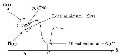
The problem can be broken down into smaller sub-problems and each sub-problem solved one at a time starting with the most difficult sub-problem.  In [19], the channel assignment problem is transformed to a graph colouring problem (another NP-complete problem [8]).  In the graph colouring  problem, a graph consists of nodes and edges (where each edge joins two nodes) and the task is to colour the nodes such that no two nodes sharing the same edge has the same colour.  The colours represent the channels and the nodes and edges represent the requirements.  The graph is divided into sub-graphs and they are ordered according to their level of assignment difficulty.  A frequency exhaustive  method is used to assign channels to each sub-graph in order of the sub-graph’s level of assignment difficulty.  The frequency exhaustive method starts by assigning the lowest numbered channel to as many requirements as possible and this is followed by the next lowest numbered channel.  The frequency exhaustive method achieves high channel packing since it gives priority to lower numbered channels.  The level of assignment difficulty can be proportional to the number of edges connected to a node (node-degree ordering) or the size of the complete sub-graph (node-colour ordering).  A complete sub-graph of size G has G nodes where each node is connected to all the other G-1 nodes (i.e. each node has G-1 edges). 

The ordering can also be done in a heuristic manner as in [20].  In this method, the base stations are ranked according to their level of “difficulty” (a value) and the ranking is done in an iterative manner.  The number of channels C is fixed and each base station is assigned a “difficulty” value, which is set to be the same at the beginning of the search.  For each iteration, channels are assigned to the base station in the order of the list.  After the channel assignment attempt for the final base station, the “difficulty” value for each base station that has call blocks  (i.e. base stations without a valid channel assignment) is increased by a random value drawn from a uniform distribution.  The list is re-sorted according to the level of difficulty and the iteration process is repeated until all the base stations have valid channels.  This method may not give the optimum solution (if C ¹ C_MIN) and the number of iterations may be large for difficult problems or may not stop if the number of channel C does not lead to a solution.

The ordering technique settles upon the first solution even if it is a poor solution (i.e. C is much greater than C_MIN).  A heuristic method that considers a set of ordered lists is considered in [21], where each list is a random order of base stations.  For each list, the algorithm assigns channels for the first base station in the list until all the traffic demand is satisfied.  The assigned channels may hinder other base stations (lower in the list) from using them since it may violate the compatibility matrix.  The algorithm will consider the next base station in the list until all base stations and their traffic demands are satisfied.  This algorithm successfully finds C_L for some problems, but for difficult problems, the algorithm may require a large number of ordered lists.

There is no measure of the cost or effectiveness of a solution in the ordering techniques.  Another approach to achieve a sub-optimal solution is to search through part of the total number of possible channel assignments.  The search space (possible channel assignments) is large and therefore the number of searches that can be performed is usually only a small fraction of the total search space.  Hence, an efficient search method is essential to find a sub-optimal solution.  A typical search method involves defining a search space S (the set of all possible solutions), where each point (possible solution) in the search space is usually represented by a matrix sÎS, a method to move from one solution s to another s’ and a cost function C(s) to give a numerical evaluation of the solution s.

An adaptive local-search method is used in [22], where an ordered list of calls is used.  An ordered list of calls is given by say, a = [a_4,1 a_5,2 a_2,3, …], where each element a_j,k represents a call (i.e. the k^th call from the base station j, each call occupies a radio transceivers).  This approach is similar to the list used in the ordering techniques in [20] and [21] described previously, but instead of having an ordered list of base stations, it has an ordered list of traffic demands (i.e., calls).  For an example, consider a set of base stations B = {b₁, b₂, b₃} with D = [3 2 2].  This means b₁ has three calls a_1,1, a_1,2 and a_1,3, b₂ has two calls a_2,1 and a_2,2; and b₃ has two calls a_3,1 and a_3,2.  If a = [a_1,3, a_2,1, a_2,2, a_1,1, a_3,1, a_3,2, a_1,2], a channel is assigned to b₁, followed by two channels to b₂, followed by one channel for b₁, then a two channels for b₃ and finally a channel for b₁.  Note that if each base station has one call demand then the nature of the lists in these three techniques ([20], [21] and [22]) are the same.  The cost C(a) is the number of channels assigned to a (ordered list of calls) using the frequency exhaustive method.  The goal is to find a call list that uses as few channels as possible to meet the traffic demand.  In a local search for each call list a, there is set of possible call lists called the neighbourhood N(a)ÎA (A is the set of all possible call lists), where each possible call list a’ÎN(a) is a slight modification of a.  For example in this case, a’ is found by swapping the orders of two calls in a.  The first a’ÎN(a) that has a lower cost (C(a’) < C(a)) replaces a (i.e. a=a’) as the next point of consideration.  This process is iterated until an estimated optimum (i.e. C(a) = C_L) solution is found or after a predefined number of iterations has taken place.  The search space of a large network can be reduced by representing a non-uniform traffic network as the superposition of two networks [22].  The first network has a uniform traffic distribution, where each base station has the minimum traffic demand of the original network.  The second network has a non-uniform traffic distribution where the traffic in each base station is the difference between the traffic of the original network and the traffic of the first network.  The first network can be solved using the method described in Figure 2.3.  The second network has a smaller search space and therefore the chance of finding an optimum solution is much greater.

Figure 2.4: Local and global minima.  A point (s, C(s)) is represented as a rolling ball.

In a search method, it is easy to get trapped in a poor local minimum, e.g. at s_l (in Figure 2.4), if C(s’) > C(s_l) for all s’ÎN(s_l) and C(s_l) > C(s*) where s* is the optimum solution (or global minimum) with the lowest cost (i.e. C(s) ³ C(s*) for all sÎS).  This can be avoided if the algorithm accepts s’ as the next transition even if C(s’) > C(s), which is equivalent to giving an upward push to the ball in Figure 2.4 so that it moves out of the valley (local minimum) to explore other regions.  In [22], this is done by accepting s’ if C(s’) ³ C(s) after a predetermined number of iterations.  Examples of algorithms that are capable of escaping from a poor local minimum are Simulated Annealing, the Tabu Search, Neural Networks (modified version) and the Genetic Algorithm.

Simulated Annealing  escapes from a poor local minimum by accepting s’ÎN(s) for C(s’) > C(s) with a probability P_sa(s’, s), which is known as the Metropolis test  and is given as:

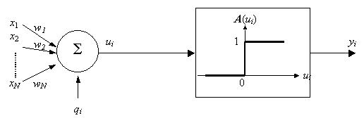
where T is the temperature.  At a high temperature the algorithm accepts more solutions with high cost and in effect it searches a large search space S, while at a low temperature the algorithm prefers solutions with low cost.  At the beginning of the iteration, the temperature is set to a high value and decreases with the number of iterations [13].  Simulated Annealing is used in [23] to find a solution for a FCA.  The solution s is a B ´ C matrix where B is the total number of base stations and C is the total number of channels and an element s_j,k in s (j=1 to B and k=1 to C) is given in equation (2.3) .  The cost C(s) encourages assignments that conform to the compatibility matrix, that meet the traffic requirement and have a high channel packing.  The neighbouring solution s’ÎN(s) is generated by replacing a used channel with a currently unused channel in base station j.

The Tabu Search  maintains a list called the Tabu List  T_LIST that contains the attributes of a solution that the algorithm has considered in past iterations.  In moving from s to s’ÎN(s), the algorithm will not select s’ if it is in the Tabu List (i.e. if s’Î T_LIST) [13].  If the size of the Tabu List ||T_LIST|| is large, the search will progress move quickly away from N(s) thereby exploring a larger search space and if || T_LIST|| is small, it will intensify its search around N(s).  The Tabu Search is used in [24], where the solution s is the same as that described in (2.3) and the neighbourhood solution s’ÎN(s) is generated in the same way as is done in the Simulated Annealing approach described previously.  However, [24] recognises and shows that the compatibility matrix is not unique for a given SIR threshold.  Rather than using a cost function, it uses a gain or a fitness function  F(s) where the aim is to maximize F(s).  For a given assignment s, F(s) is the number of channels assigned to a base station that have a SIR above a predefined threshold, where the SIR takes into account the cumulative interference from all co-channel base stations.

A popular method employed to solve the FCA problem is the Neural Network.  A neuron in a Neural Network  is shown in Figure 2.5, where x = [x₁, x₂, … x_N] is the input and q_i is a bias current for neuron i [14].  The internal state u_i of neuron i is given by:

where w_j is the weight for input x_j.  The activation function A(u_i) is a function of the internal state u_i and is usually 0 £ A(u_i) £ 1 (e.g. a unit step function) and the output of neuron i is y_i= A(u_i).

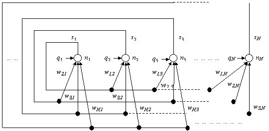
Figure 2.5: Representation of neuron i.

In a Hopfield Neural Network  (HNN) [15], the output of all neurons are connected to the input of every other neuron except itself.  This is shown in Figure 2.6, where x=[x₁, x₂, …, x_N] is the output from the neurons, x_i is the output of neuron i (i.e. n_i) and w_j,k is the weight from n_j to n_k (which weights x_j prior to entering neuron n_k)  The weights in a HNN are symmetrical (w_j,k = w_k,j) and w_j,j = 0.  The state of each neuron is its current output x_jÎ{0,1} and the energy E(x) in the HNN decreases for each update of x until it converges to a local minimum, which is dependent upon the weights.  Hence, by constructing an appropriate E(x) corresponding to the cost of an optimisation problem and expressing the state of the neuron x as a possible solution, a HNN with the appropriate weights can find a solution to an optimisation problem.

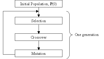
Figure 2.6: Hopfield Neural Network (a black solid dot represents a connection).

In [25], a HNN is used to find a sub-optimal solution for FCA.  Here, a neuron is an element s_j,k in s (j=1 to B and k=1 to C) as in (2.3) giving B ´ C neurons.  The energy E(s) is equivalent to the cost function C(s) and w_{j,k,j’,k’} is the weight from neuron s_j,k to neuron s_j’,k’ and it is a function of the interference between s_j,k and s_j’,k’.  The weight w_{j,k,j’,k’} decreases if the channel separation |k - k’| < c_j,j’ Î C (the channel separation between base station j and j’ in the compatibility matrix).  The bias current q_j is proportional to the traffic demand of base station j yielding an energy E(s) that is a function of the overall interference of the network and the traffic supported for a given assignment s.  A HNN minimising E(s) is equivalent to finding a solution s with a low cost C(s).

The HNN technique is not able to escape from a local minimum and realising this an improved HNN is used in [26] where a temporary increase in E(s) is permitted so that it can escape from local minima.  The increase in E(s) is achieved by introducing noise via a random function into the internal function u_i in (2.8) .  This will change the value of A(u_i), thereby causing a random increase in E(s).  The random increase in E(s) becomes less as time proceeds in a similar way to the process employed in Simulated Annealing.

The Genetic Algorithm  [16] is inspired by the natural process of the adaptation of species in an environment.  Instead of a neighbourhood N(s) of possible solutions centred around s as in Simulated Annealing and Tabu Search, the Genetic Algorithm considers a population  P(t)ÎS, which is a set of possible solutions where at the t^th iteration, P(t)={s₁, s₂, … s_K}, where K = |P(t)|.  Hence, the Genetic Algorithm searches various points in S rather than those centred around N(s).  Each solution sÎP(t) is called an individual and it is evaluated using a fitness function  F(s), which measures the gain of using solution s in a similar way to the cost function C(s).  Using F(s) the optimum solution is the global maximum as compared to C(s) where the optimum solution is the global minimum.  The Genetic Algorithm starts off with an initial population P(0) and it is followed by  Selection, Crossover and Mutation processes.  These processes are shown in Figure 2.7.

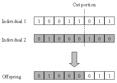
Figure 2.7: Processes in a Genetic Algorithm.

In the Selection  process, individuals are selected for the Crossover process where individuals with a higher fitness F(s) have a higher probability of being selected.  Figure 2.8 shows the Crossover  process with two individuals, where a portion of Individual 1 is cut and placed into the same portion of Individual 2 to produce a new individual (the offspring).  The two individuals selected have a probability of p_c of being subjected to Crossover. 

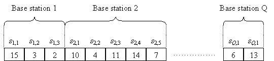
Figure 2.8: Crossover process.

In the Mutation  process, each element in an individual is changed (in the case of binary representation, the element is complemented) with a small probability of p_m.  These 3 processes are performed on P(t) to produce a new generation of individuals P(t+1).  Although Selection favours fitter individuals, individuals with poor fitness also have a chance of being selected so that the algorithm will not converge to a poor local maximum.  The average fitness of the population will increase and converge after a number of generations (i.e., iterations) as the individuals in the population become more similar to each other.  Mutation  increases diversity in the population and thus allows the algorithm to search more distinct points.

The Genetic Algorithm is applied to the FCA problem for both uniform and non-uniform traffic in [27].  The size of string  s is equal to the sum of the traffic demand for all base stations, and each element s_j,k in s is a channel number that is assigned to base station j for the k^th call.  This is illustrated in Figure 2.9.  The traffic demand for each base station is included in the structure of the string and therefore the fitness function consists only of the co-channel and adjacent channel constraints.

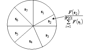
Figure 2.9: String representation s of an individual.

Roulette wheel  selection is used in [27], where each section in the wheel corresponds to an individual and the size of each section is proportional to the individual’s fitness.  This is illustrated in Figure 2.10.  Selection is random but biased towards individuals with a higher fitness.  The probability of being selected is shown in Figure 2.10.

Figure 2.10: Roulette wheel selection – section size proportional to fitness (shown here for s₂).

The Genetic Algorithm is used in [28] to search for an ordered call list a instead of an assignment.  The call list a is the same as that used in the local search method [22] described previously.  As in [22], a frequency exhaustive method is used to assign channels to a.  However, in [28] the number of channels C is given and the fitness is a function of the number of blocked calls (i.e. the number of calls without valid assignments) and the degree of channel packing.  To find the C_MIN, this method first uses an estimated lower bound for C and if the algorithm fails to find a solution (i.e. one with no blocked calls) within a predefined number of iterations it increases C and restarts the algorithm.  This method also uses roulette wheel selection depicted in Figure 2.10. 

All the methods described are able to find a solution satisfying the compatibility matrix if the given number of channels C is larger than C_MIN.  However, for a given compatibility matrix, if C < C_MIN, no solution exists to the channel allocation problem without giving rise to call blocks.  Rather than having a hard constraint (i.e. conforming fully to the compatibility matrix), a soft constraint that allows a channel assignment to violate the compatibility matrix can be applied to guarantee a solution at the expense of higher interference.  In applying a soft constraint,  a violation with a higher channel separation is preferred to one with a smaller channel separation.  For example if two base stations require a channel separation of 5 and no channel allocation can satisfy this, it is preferable to select an assignment with a channel separation of 4 compared with one with a channel separation of 2.  However, if the channel separation condition is satisfied then in order to achieve higher channel packing, it is preferred to have an assignment with a channel separation of 5 than one with a channel separation of 7.  If C > C_MIN applying a soft constraint may produce a solution with high interference if the solution is trapped in a bad local minimum.  The energy function used in the improved HNN in [26] implements a soft constraint on the compatibility matrix and a hard constraint on the traffic demand.  A soft constraint is also implemented into the cost function of the Simulated Annealing technique in [23].  A soft constraint is also used in [29], where the network is divided in groups of cells and in each group, the cells are further grouped into co-channel sub-groups.  For each co-channel sub-group in a cluster, channels are assigned to the cell with the highest traffic demand.  The remainder of the cells in the co-channel sub-group can thus use these channels.  For cells that do not belong to any co-channel sub-group, and if no channel that conforms to the interference constraint is found, a soft constraint is applied where up to 13% of interference power is allowed to exceed the required minimum.

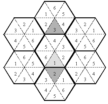
Figure 2.11: Time slots arrangement in SRA (numbers indicate time slot number).

Most of the FCAs considered are used for mobile cellular communication.  In [30] a Channel Allocation method called Staggered Resource Allocation  (SRA) is introduced for use in a Broadband Fixed Wireless Access  Network where the spectrum is reused in every cell.  For a frequency reuse of one, the cells are divided into sectors where each base station uses a sectored antenna.  The SRA method uses TDMA and ensures that base stations with the front lobe of the antenna pointing towards each other do not transmit at the same time.  Consider the cell layout shown in Figure 2.11, where the system has six time slots in a TDMA frame and six sectors in each cell.