Exercises for the second supervision

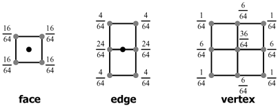
1. The Doo-Sabin subdivision scheme is illustrated in SMEG, page 23, Figure 3. The Reif-Peters scheme is illustrated in the diagram on the right. Reif-Peters uses a different approach to Doo-Sabin: in it the new points are generated halfway between existing points and connected up into a mesh as illustrated in the diagram on the right (black: original mesh; grey: new mesh). Note that (i) the existing points do not form part of the new mesh and (ii) each new point's position is simply the average of the positions of the two existing points at either end of the corresponding line segment.
   (a) Doing the Reif-Peters subdivision twice produces a mesh which looks similar to that produced by doing the Doo-Sabin subdivision once (SMEG, page 23, Figure 3(left)). You can treat two steps of Reif-Peters as if it were a single step of a Doo-Sabin-like subdivision scheme. Calculate the weights on the original points for each new point after two steps of Reif-Peters (i.e. work out what numbers replace those in SMEG Figure 3(right) for the Reif-Peters two step scheme). [2 marks]
   (b) For the Reif-Peters one step scheme, explain what happens around extraordinary vertices and what happens around extraordinary polygons, giving examples. [2 marks]
2. [2003 P7 Q4 (c)] The Catmull-Clark bivariate subdivision scheme is a bivariate generalisation of the univariate 1/8 [1, 4, 6, 4, 1] subdivision scheme. It creates new vertices as blends of old vertices in the following ways:
   
   (i) Provide similar diagrams for the bivariate generalisation of the univariate four-point interpolating subdivision scheme 1/16 [-1, 0, 9, 16, 9, 0,-1]. [5 marks]
   (ii) Explain what problems arise around extraordinary vertices (vertices of valency other than four) for this bivariate interpolating scheme and suggest a possible way of handling the creation of new edge vertices when the old vertex at one end of the edge has a valency other than four. [4 marks]
3. There is a univariate binary C2 6-point subdivision scheme which interpolates the original points and generates a new point between every existing pair by:
   P_2iⁿ⁺¹=P_iⁿ
   P_2i+1ⁿ⁺¹= a₀P_i-2ⁿ + a₁P_i-1ⁿ + a₂P_iⁿ + a₃P_i+1ⁿ + a₄P_i+2ⁿ + a₅P_i+3ⁿ
   There is also a univariate ternary C2 4-point subdivision scheme which interpolates the original points and generates two new points between every exisiting pair by:
   P_3iⁿ⁺¹=P_iⁿ
   P_3i+1ⁿ⁺¹= c₀P_i-1ⁿ + c₁P_iⁿ + c₂P_i+1ⁿ + c₃P_i+2ⁿ
   P_3i+2ⁿ⁺¹= c₃P_i-1ⁿ + c₂P_iⁿ + c₁P_i+1ⁿ + c₀P_i+2ⁿ
   The actual values of a_i and c_i need not concern us for the purposes of this exercise.
   (a) Given an initial set (n=0) with M points, how many floating point operations (additions and multiplications) are required in the binary and ternary cases to create the complete set of points for n=1? For both binary and ternary, consider both the case of a closed curve and the case of an open curve. (Notes: (1) in an open curve, we only generate a new point if all the old points needed to calculate it actually exist; (2) in a closed curve, the two ends of the curve join up and where we need points which fall off the end of the sequence of points we can simply loop round the indices by saying P_iⁿ=P_i+Mⁿ.) [4 marks]
   (b) Both methods produce a C2 interpolating limit curve. We want to compare the methods by producing refined sets of control points using each of the two methods and compare the number of calculations involved to see which is more efficient. Obviously we cannot get exactly the same number of points in the refined sets [why not?]. So, say we produce a refined set of points with (roughly) 8 times (binary) or 9 times (ternary) as many points as in the original, then which of the two methods is more efficient in terms of number of floating point operations? [2 marks]
   (c) For large M, what factors other than number of floating point operations will affect execution speed? How does execution speed depend on M? [3 marks]
   
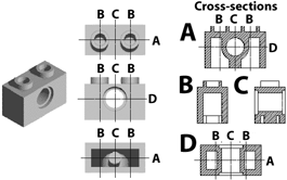
4. [2003 P9 Q6 (c)] Show how the following object can be constructed using Constructive Solid Geometry (CSG). You may assume the following primitives: sphere, cylinder, cone, torus, box. [You are expected to describe which primitives are needed and how they are combined but you are not expected to specify accurately all of the parameters of the primitives.] [4 marks]
   
   
5. [4C/3] List the three ways of combining objects using constructive solid geometry (CSG). Describe how an object built using CSG can be represented using a binary tree. Given the intersection points of a ray with each primitive in the tree, explain how these points are passed up the tree by each type of combination node to produce a list of intersection points for the whole CSG object. [8 marks]
6. [4D/4] The marching squares algorithm is a two-dimensional version of marching cubes, where you generate line segments in 2D rather than triangles in 3D. It could be used, for example, where you have a regular grid of height values and want to draw contours of constant height. Sketch an implementation of this two-dimensional marching squares algorithm. [6 marks]