The Quantized Degrees-of-Freedom in a Continuous Signal

There are several important results in continuous mathematics expressing the idea that even though a function (such as some time-varying signal) is continuous and dense in time (i.e. the value of the signal is defined at each real-valued moment in time), nevertheless a finite and countable set of discrete numbers suffices to describe it completely, and thus to reconstruct it, provided that its frequency bandwidth is limited.

Such theorems may seem counter-intuitive at first: How could a finite sequence of numbers, at discrete intervals, capture exhaustively the continuous and uncountable stream of numbers that represent all the values taken by a signal over some interval of time?

In general terms, the reason is that bandlimited continuous functions are not as free to vary as they might at first seem. Consequently, specifying their values at only certain points, suffices to determine their values at all other points.

 

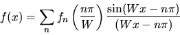
Figure 2: The sinc function for recovering a continuous signal exactly from its discrete samples, provided their frequency equals the Nyquist rate.

Some examples are:

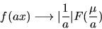
• Nyquist's Sampling Theorem: If a signal f(x) is strictly bandlimited so that it contains no frequency components higher than W, i.e. its Fourier Transform $F(\mu)$ satisfies the condition
  

  $$F(\mu) = 0 {\rm\hspace*{0.05in}for\hspace*{0.05in}} \vert\mu\vert > W$$ (69)

  
  
  then f(x) is completely determined just by sampling its values at a rate of at least 2W. The signal f(x) can be exactly recovered by using each sampled value to fix the amplitude of a sinc(x) function,
  

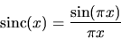  $${\rm sinc}(x) = \frac{ \sin (\pi x)}{\pi x}$$ (70)

  
  
  whose width is scaled by the bandwidth parameter W and whose location corresponds to each of the sample points. The continuous signal f(x)can be perfectly recovered from its discrete samples $f_{n}(\frac{n\pi}{W})$just by adding all of those displaced sinc(x) functions together, with their amplitudes equal to the samples taken:
  

  $$f(x)=\sum_{n} f_{n}\left(\frac{n\pi}{W}\right)\frac{\sin(Wx-n\pi)}{(Wx-n\pi)}$$ (71)

  
  
  (The Figure illustrates this function.) Thus, any signal that is limited in its bandwidth to W, during some duration Thas at most 2WT degrees-of-freedom. It can be completely specified by just 2WT real numbers!

• The Information Diagram: The Similarity Theorem of Fourier Analysis asserts that if a function becomes narrower in one domain by a factor a, it necessarily becomes broader by the same factor a in the other domain:
  

  $$f(x) \longrightarrow F(\mu)$$ (72)

  
  
  
  

  $$f(ax) \longrightarrow \vert \frac{1}{a} \vert F(\frac{\mu}{a})$$ (73)

  
  
  The Hungarian Nobel-Laureate Dennis Gabor took this principle further with great insight and with implications that are still revolutionizing the field of signal processing (based upon wavelets), by noting that an Information Diagram representation of signals in a plane defined by the axes of time and frequency is fundamentally quantized. There is an irreducible, minimal, volume that any signal can possibly occupy in this plane. Its uncertainty (or spread) in frequency, times its uncertainty (or duration) in time, has an inescapable lower bound.

Gabor-Heisenberg-Weyl Uncertainty Relation. ``Logons."

The Uncertainty Principle

If we define the ``effective support" of a function f(x) by its normalized variance, or the normalized second-moment

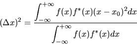$$(\Delta x)^{2} = \frac{\displaystyle \int_{-\infty}^{+\infty}... ... dx} {\displaystyle \int_{-\infty}^{+\infty} f(x) f^{*}(x) dx}$$ (74)

where x₀ is the mean value, or first-moment, of the function

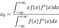$$x_{0} = \frac{\displaystyle \int_{-\infty}^{+\infty} x f(x) f... ...dx } {\displaystyle \int_{-\infty}^{+\infty} f(x) f^{*}(x) dx}$$ (75)

and if we similarly define the effective support of the Fourier Transform $F(\mu)$ of the function by its normalized variance in the Fourier domain

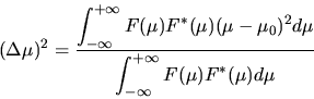$$(\Delta \mu)^{2} = \frac{\displaystyle \int_{-\infty}^{+\inft... ...\displaystyle \int_{-\infty}^{+\infty} F(\mu) F^{*}(\mu) d\mu}$$ (76)

where $\mu_{0}$ is the mean value, or first-moment, of the Fourier transform $F(\mu)$

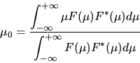$$\mu_{0} = \frac{\displaystyle \int_{-\infty}^{+\infty} \mu F(... ...\displaystyle \int_{-\infty}^{+\infty} F(\mu) F^{*}(\mu) d\mu}$$ (77)

then it can be proven (by Schwartz Inequality arguments) that there exists a fundamental lower bound on the product of these two ``spreads," regardless of the function f(x) !

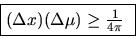$$\fbox{$(\Delta x) (\Delta \mu) \ge \frac{1}{4 \pi} $\space }$$ (78)

This is the famous Gabor-Heisenberg-Weyl Uncertainty Principle. Mathematically it is exactly identical to the uncertainty relation in quantum physics, where $(\Delta x)$ would be interpreted as the position of an electron or other particle, and $(\Delta \mu)$ would be interpreted as its momentum or deBroglie wavelength. We see that this is not just a property of nature, but more abstractly a property of all functions and their Fourier Transforms. It is thus a still further, and more lofty, respect in which the information in continuous signals is quantized, since they must occupy an area in the Information Diagram (time - frequency axes) that is always greater than some irreducible lower bound.

Gabor ``Logons"

Dennis Gabor named such minimal areas ``logons" from the Greek word for information, or order: logos. He thus established that the Information Diagram for any continuous signal can contain only a fixed number of information ``quanta." Each such quantum constitutes an independent datum, and their total number within a region of the Information Diagram represents the number of independent degrees-of-freedom enjoyed by the signal.

The unique family of signals that actually achieve the lower bound in the Gabor-Heisenberg-Weyl Uncertainty Relation are the complex exponentials multiplied by Gaussians. These are sometimes referred to as ``Gabor wavelets:"

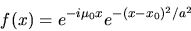$$f(x)=e^{-i \mu_{0} x} e^{-(x-x_{0})^{2}/a^{2} }$$ (79)

localized at ``epoch" x₀, modulated by frequency $\mu_{0}$, and with size or spread constant a. It is noteworthy that such wavelets have Fourier Transforms $F(\mu)$ with exactly the same functional form, but with their parameters merely interchanged or inverted:

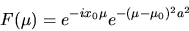$$F(\mu)=e^{-i x_{0} \mu} e^{-(\mu-\mu_{0})^{2}a^{2} }$$ (80)

Note that in the case of a wavelet (or wave-packet) centered on x₀=0, its Fourier Transform is simply a Gaussian centered at the modulation frequency $\mu_{0}$, and whose size is 1/a, the reciprocal of the wavelet's space constant.

Because of the optimality of such wavelets under the Uncertainty Principle, Gabor (1946) proposed using them as an expansion basis to represent signals. In particular, he wanted them to be used in broadcast telecommunications for encoding continuous-time information. He called them the ``elementary functions" for a signal. Unfortunately, because such functions are mutually non-orthogonal, it is very difficult to obtain the actual coefficients needed as weights on the elementary functions in order to expand a given signal in this basis! The first constructive method for finding such ``Gabor coefficients" was developed in 1981 by the Dutch physicist Martin Bastiaans, using a dual basis and a complicated non-local infinite series.

When a family of such functions are parameterized to be self-similar, i.e. they are dilates and translates of each other so that they all have a common template (``mother" and ``daughter"), then they constitute a (non-orthogonal) wavelet basis. Today it is known that an infinite class of wavelets exist which can be used as the expansion basis for signals. Because of the self-similarity property, this amounts to representing or analyzing a signal at different scales. This general field of investigation is called multi-resolution analysis.

Two-dimensional Gabor filters over the image domain (x,y) have the functional form

$$f(x,y)=e^{-\left[(x-x_{0})^{2}/\alpha^{2} + (y-y_{0})^{2}/\beta^{2}\right]} e^{-i\left[u_{0}(x-x_{0}) + v_{0}(y-y_{0})\right]}$$ (81)

where (x₀,y₀) specify position in the image, $(\alpha, \beta)$ specify effective width and length, and (u₀,v₀) specify modulation, which has spatial frequency $\omega_{0}=\sqrt{u_{0}^{2}+v_{0}^{2}}$and direction $\theta_{0}=\arctan(v_{0}/u_{0})$. (A further degree-of-freedom not included above is the relative orientation of the elliptic Gaussian envelope, which creates cross-terms in xy.) The 2-D Fourier transform F(u,v) of a 2-D Gabor filter has exactly the same functional form, with parameters just interchanged or inverted:

$$F(u,v)=e^{-\left[(u-u_{0})^{2}\alpha^{2} + (v-v_{0})^{2}\beta^{2}\right]} e^{-i\left[x_{0}(u-u_{0}) + y_{0}(v-v_{0})\right]}$$ (82)

2-D Gabor functions can form a complete self-similar 2-D wavelet expansion basis, with the requirements of orthogonality and strictly compact support relaxed, by appropriate parameterization for dilation, rotation, and translation. If we take $\Psi(x,y)$ to be a chosen generic 2-D Gabor wavelet, then we can generate from this one member a complete self-similar family of 2-D wavelets through the generating function:

$$\Psi_{mpq\theta}(x,y)=2^{-2m}\Psi(x',y')$$ (83)

where the substituted variables (x',y') incorporate dilations in size by 2^-m, translations in position (p,q), and rotations through orientation $\theta$:

$$x'=2^{-m}[x\cos(\theta) + y\sin(\theta)]-p$$ (84)

$$y'=2^{-m}[-x\sin(\theta)+y\cos(\theta)]-q$$ (85)

It is noteworthy that as consequences of the similarity theorem, shift theorem, and modulation theorem of 2-D Fourier analysis, together with the rotation isomorphism of the 2-D Fourier transform, all of these effects of the generating function applied to a 2-D Gabor mother wavelet $\Psi(x,y) = f(x,y)$ have corresponding identical or reciprocal effects on its 2-D Fourier transform F(u,v). These properties of self-similarity can be exploited when constructing efficient, compact, multi-scale codes for image structure.

Grand Unification of Domains: an Entente Cordiale

Now we can see that the ``Gabor domain" of representation actually embraces and unifies both the Fourier domain and the original signal domain! To compute the representation of a signal or of data in the Gabor domain, we find its expansion in terms of elementary functions having the form

$$f(x)=e^{-i \mu_{0} x} e^{-(x-x_{0})^{2}/a^{2} }$$ (86)

The single parameter a (the space-constant in the Gaussian term) actually builds a continuous bridge between the two domains: if the parameter a is made very large, then the second exponential above approaches 1.0, and so in the limit our expansion basis becomes

$$\lim_{a \rightarrow \infty} f(x)=e^{-i \mu_{0} x}$$ (87)

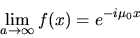
the ordinary Fourier basis! If the parameter a is instead made very small, the Gaussian term becomes the approximation to a delta function at location x_o, and so our expansion basis implements pure space-domain sampling:

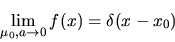$$\lim_{\mu_{0},a \rightarrow 0} f(x)=\delta(x-x_{0})$$ (88)

Hence the Gabor expansion basis ``contains" both domains at once. It allows us to make a continuous deformation that selects a representation lying anywhere on a one-parameter continuum between two domains that were hitherto distinct and mutually unapproachable. A new Entente Cordiale, indeed.