Exercises for the second supervision

For your convenience the set of exercises is gathered together below.

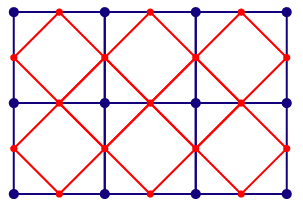
• [New] The Doo-Sabin subdivision scheme is illustrated in SMEG, page 23, Figure 3. The Reif-Peters scheme is illustrated in the diagram on the right. Reif-Peters uses a different approach to Doo-Sabin: in it the new points are generated halfway between existing points and connected up into a mesh as illustrated in the diagram on the right (blue: original mesh; red: new mesh). Note that (i) the existing points do not form part of the new mesh and (ii) each new point's position is simply the average of the positions of the two existing points at either end of the corresponding line segment.
  (a) Doing the Reif-Peters subdivision twice produces a mesh which looks similar to that produced by doing the Doo-Sabin subdivision once (SMEG, page 23, Figure 3(left)). You can treat two steps of Reif-Peters as if it were a single step of a Doo-Sabin-like subdivision scheme. Calculate the weights on the original points for each new point after two steps of Reif-Peters (i.e. work out what numbers replace those in SMEG Figure 3(right) for the Reif-Peters two step scheme). [2 marks]
  (b)For the Reif-Peters one step scheme, explain what happens around extraordinary vertices and what happens around extraordinary polygons, giving examples. [2 marks]
• New The univariate binary C2 6-point subdivision scheme interpolates the original points and generates a new point between every existing pair by:
  P_2iⁿ⁺¹=P_iⁿ
  P_2i+1ⁿ⁺¹= a₀P_i-2ⁿ + a₁P_i-1ⁿ + a₂P_iⁿ + a₃P_i+1ⁿ + a₄P_i+2ⁿ + a₅P_i+3ⁿ
  The univariate ternary C2 4-point subdivision scheme interpolates the original points and generates two new points between every exisiting pair by:
  P_3iⁿ⁺¹=P_iⁿ
  P_3i+1ⁿ⁺¹= c₀P_i-1ⁿ + c₁P_iⁿ + c₂P_i+1ⁿ + c₃P_i+2ⁿ
  P_3i+2ⁿ⁺¹= c₃P_i-1ⁿ + c₂P_iⁿ + c₁P_i+1ⁿ + c₀P_i+2ⁿ
  (a) Given an initial set (n=0) with M points, how many floating point operations are required in the binary and ternary cases to create the complete set of points for n=1? For both binary and ternary, consider both the case of an open curve and the case of a closed curve. (Note: in a closed curve the two ends of the curve join up and where we need points which fall off the end of the sequence of points we can simply loop round the indices by saying P_iⁿ=P_i+Mⁿ.) [4 marks]
  (b) Both methods produce a C2 interpolating limit curve. We want to compare the methods by producing refined sets of control points using each of the two methods and compare the number of calculations involved to see which is more efficient. Obviously we cannot get exactly the same number of points in the refined sets (why not?). So, say we produce a refined set of points with (roughly) 8 times (binary) or 9 times (ternary) as many points as in the original, then which of the two methods is more efficient in terms of floating point operations? [2 marks]
  (c) What factors other than number of floating point operations will affect execution speed? How does execution speed depend on M? [3 marks]
  (d) Now, distribute the original set of points evenly along the x-axis, with P_i⁰=(i,0) for all i, except P₀⁰=(0,1). In the limit, most of the limit curve will lie exactly on the x-axis. For both the binary and the ternary scheme, what is the range of values of x for which the limit curve does not lie on the x-axis? Assume that a_j≠0, j ∈ {0,1,2,3,4,5} and c_j≠0, j ∈ {0,1,2,3}. (Note: the point of doing this is that it tells you how much of the limit curve is affected if you move a single original point.) [4 marks]
• [4A/3] For each of the following categories list five real-world objects which could be represented by the primitives in the category.
  1. The ray-tracing primitives in Part 2A
  2. Extrusions
  3. Surfaces of revolution
  4. General sweeps (generalised cylinders) which cannot be represented by just an extrusion or a surface of revolution.
  [4 marks]
• [4C/3] List the three ways of combining objects using constructive solid geometry (CSG). Describe how an object built using CSG can be represented using a binary tree. Given the intersection points of a ray with each primitive in the tree, explain how these points are passed up the tree by each type of combination node to produce a list of intersection points for the whole CSG object. [8 marks]
• [4D/4] The marching squares algorithm is a two-dimensional version of marching cubes, where you generate line segments in 2D rather than triangles in 3D. It could be used, for example, where you have a regular grid of height values and want to draw contours of constant height. Sketch an implementation of this two-dimensional marching squares algorithm. [6 marks]
• [5/2] Explain what a form factor is, in radiosity. Outline an implementable method of calculating form factors. [5 marks]