Exercises for the second supervision

• [6.4/5(d)] Show that the B-spline with k = 2 and knot vector [ 0 0 0 1 1 1 ] is equivalent to the quadratic Bezier curve.
• Give a knot vector and value of k which would desribe a uniform B-spline equivalent to a cubic Bezier curve.
• [6.4/6] Derive the formula of and sketch a graph of N_3,2(t), the third of the quadratic B-spline basis functions, for the knot vector [ 0 0 0 1 3 3 4 5 5 5 ].
• Give the coeffcient polynomials for a bivariate quadratic triangular Bezier patch. This was not covered in lecture: you will have to do a little research. (Or derive them from first principles, of course.) Be sure that your answer is truly bivariate (only two varying parameters) and please cite your sources where apropriate.
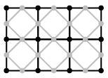• The Doo-Sabin subdivision scheme is illustrated in the lecture notes in Figure 19 (in 2007, Figure 18 in the 2006 notes). The Reif-Peters scheme is illustrated in the diagram on the right. Reif-Peters uses a different approach to Doo-Sabin: in it the new points are generated halfway between existing points and connected up into a mesh as illustrated in the diagram on the right (black: original mesh; grey: new mesh). Note that (i) the existing points do not form part of the new mesh and (ii) each new point's position is simply the average of the positions of the two existing points at either end of the corresponding line segment.
  (a) Doing the Reif-Peters subdivision twice produces a mesh which looks similar to that produced by doing the Doo-Sabin subdivision once (Figure 19(left)). You can treat two steps of Reif-Peters as if it were a single step of a Doo-Sabin-like subdivision scheme. Calculate the weights on the original points for each new point after two steps of Reif-Peters (i.e. work out what numbers replace those in Figure 19(right) for the Reif-Peters two step scheme).
  (b) For the Reif-Peters one step scheme, explain what happens around extraordinary vertices and what happens around extraordinary polygons, giving examples.
• [2003 P7 Q4 (c)] The Catmull-Clark bivariate subdivision scheme is a bivariate generalisation of the univariate 1/8 [1, 4, 6, 4, 1] subdivision scheme. It creates new vertices as blends of old vertices in the following ways:
  
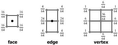
  (i) Provide similar diagrams for the bivariate generalisation of the univariate four-point interpolating subdivision scheme 1/16 [-1, 0, 9, 16, 9, 0,-1].
  (ii) Explain what problems arise around extraordinary vertices (vertices of valency other than four) for this bivariate interpolating scheme and suggest a possible way of handling the creation of new edge vertices when the old vertex at one end of the edge has a valency other than four.
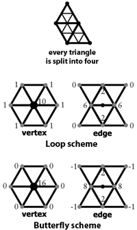• [2004 P7 Q4 (c)] The Loop and Butterfly subdivision schemes can both operate on triangular meshes, in which all of the polygons have three sides. Both schemes subdivide the mesh by introducing new vertices at the midpoints of edges, splitting every original triangle into four smaller triangles, as shown at right. Each scheme has rules for calculating the locations of the new "edge" and "vertex" vertices based on the locations of the old vertices. These rules are shown at right. All weights should be multiplied by 1/16.
  (i) Which of the two schemes produces a limit surface which interpolates the original data points?
  (ii) Which of the four rules must be modified when there is an extraordinary vertex? For each of the four rules either explain why it must be modified or explain why it does not need to be modified.
  (iii) Suggest appropriate modifications where necessary to accommodate extraordinary vertices.
• [8.3.3/3] The marching squares algorithm is a two-dimensional version of marching cubes, where processing iterates over intelligently-chosen four-sided squares instead of six-sided cubes. Sketch an implementation of this two-dimensional algorithm; be sure to mention how you will ensure that small, isolated pieces of the surface are not lost in processing.
• Explain the special cases in the polygonalization of an octree, and how you might address them.