|
Exercises for the second supervision
 The Doo-Sabin subdivision scheme is
illustrated in the lecture notes in Figure 19 (in 2007, Figure 18 in
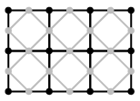
the 2006 notes). The Reif-Peters scheme is illustrated in the diagram
on the right. Reif-Peters uses a different approach to Doo-Sabin: in
it the new points are generated halfway between existing points and
connected up into a mesh as illustrated in the diagram on the right
(black: original mesh; grey: new mesh). Note that (i) the existing
points do not form part of the new mesh and (ii) each new point's
position is simply the average of the positions of the two existing
points at either end of the corresponding line segment. The Doo-Sabin subdivision scheme is
illustrated in the lecture notes in Figure 19 (in 2007, Figure 18 in
the 2006 notes). The Reif-Peters scheme is illustrated in the diagram
on the right. Reif-Peters uses a different approach to Doo-Sabin: in
it the new points are generated halfway between existing points and
connected up into a mesh as illustrated in the diagram on the right
(black: original mesh; grey: new mesh). Note that (i) the existing
points do not form part of the new mesh and (ii) each new point's
position is simply the average of the positions of the two existing
points at either end of the corresponding line segment.
(a)
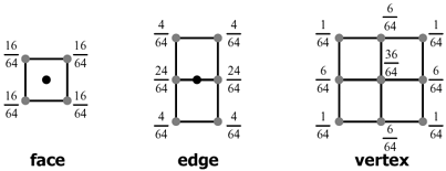
Doing the Reif-Peters subdivision twice produces a mesh which looks
similar to that produced by doing the Doo-Sabin subdivision once
(Figure 19(left)). You can treat two steps of Reif-Peters as if it
were a single step of a Doo-Sabin-like subdivision scheme. Calculate
the weights on the original points for each new point after two steps
of Reif-Peters (i.e. work out what numbers replace those in Figure
19(right) for the Reif-Peters two step scheme). [2 marks]
(b) For the Reif-Peters one step scheme, explain what happens around
extraordinary vertices and what happens around extraordinary polygons,
giving examples. [2 marks]- [2003 P7 Q4 (c)] The Catmull-Clark bivariate subdivision
scheme is a bivariate generalisation of the univariate 1/8 [1, 4, 6,
4, 1] subdivision scheme. It creates new vertices as blends of old
vertices in the following ways:

(i) Provide similar diagrams for the bivariate generalisation of the univariate
four-point interpolating subdivision scheme 1/16 [-1, 0, 9, 16, 9, 0,-1].
[5 marks]
(ii) Explain what problems arise around extraordinary vertices (vertices of
valency other than four) for this bivariate interpolating scheme and
suggest a possible way of handling the creation of new edge vertices when
the old vertex at one end of the edge has a valency other than four.
[4 marks]
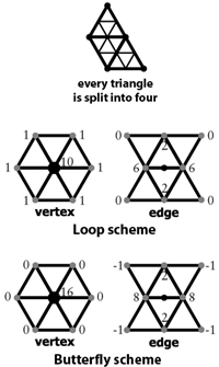
 [2004 P7 Q4 (c)] The Loop and
Butterfly subdivision schemes can both operate on triangular meshes,
in which all of the polygons have three sides. Both schemes subdivide
the mesh by introducing new vertices at the midpoints of edges,
splitting every original triangle into four smaller triangles, as
shown at right. Each scheme has rules for calculating the locations of
the new "edge" and "vertex" vertices based on the locations of the old
vertices. These rules are shown at right. All weights should be
multiplied by 1/16. [2004 P7 Q4 (c)] The Loop and
Butterfly subdivision schemes can both operate on triangular meshes,
in which all of the polygons have three sides. Both schemes subdivide
the mesh by introducing new vertices at the midpoints of edges,
splitting every original triangle into four smaller triangles, as
shown at right. Each scheme has rules for calculating the locations of
the new "edge" and "vertex" vertices based on the locations of the old
vertices. These rules are shown at right. All weights should be
multiplied by 1/16.
(i) Which of the two schemes produces a limit surface which
interpolates the original data points?
(ii) Which of the four rules
must be modified when there is an extraordinary vertex? For each of
the four rules either explain why it must be modified or explain why
it does not need to be modified.
(iii) Suggest appropriate
modifications where necessary to accommodate extraordinary vertices.
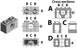
[9 marks]- [2003 P9 Q6 (c)] Show how the following object can be
constructed using Constructive Solid Geometry (CSG). You may assume
the following primitives: sphere, cylinder, cone, torus, box. [You are
expected to describe which primitives are needed and how they are
combined but you are not expected to specify accurately all of the
parameters of the primitives.] [4 marks]

- [8.8.2/3] List the three ways of combining objects using
constructive solid geometry (CSG). Describe how an object built using
CSG can be represented using a binary tree. Given the intersection
points of a ray with each primitive in the tree, explain how these
points are passed up the tree by each type of combination node to
produce a list of intersection points for the whole CSG object. [8
marks]
- [8.8.2/5] Write an ML function, similar to that in Figure 34, which finds the difference of two objects, A\B. [5 marks].
- [8.3.3/3] The marching squares algorithm is a
two-dimensional version of marching cubes, where you generate line
segments in 2D rather than triangles in 3D. It could be used, for
example, where you have a regular grid of height values and want to
draw contours of constant height. Sketch an implementation of this
two-dimensional marching squares algorithm. [6 marks]
- [1999 P9 Q4 (d)] Explain what a form factor is, in
radiosity. Outline an implementable method of calculating form
factors.
This exercise set is marked out of 50. This should take 90
minutes in an examination.
|