Algorithmic Differentiation
Algorithmic differentiation (AD) is also known as automatic differentiation. It is a powerful tool in many fields, especially useful for fast prototyping in machine learning research. Comparing to numerical differentiation which can only provides approximate results, AD can calculates the exact derivative of a given function.
Owl provides both numerical differentiation (in Numdiff.Generic module) and algorithmic differentiation (in Algodiff.Generic module). In this chapter, I will only go through AD module since Numerical module is trivial to use.
High-level APIs
Algodiff.Generic is a functor which is able to support both float32 and float64 precision AD. However, you do not need to deal with Algodiff.Generic.Make directly since there are already two ready-made modules.
Algodiff.Ssupportsfloat32precision;Algodiff.Dsupportsfloat64precision;
Algodiff has implemented both forward and backward mode of AD. The complete list of APIs can be found in owl_algodiff_generic.mli. The core APIs are listed below.
val diff : (t -> t) -> t -> t
(* calculate derivative for f : scalar -> scalar *)

val grad : (t -> t) -> t -> t
(* calculate gradient for f : vector -> scalar *)

val jacobian : (t -> t) -> t -> t
(* calculate jacobian for f : vector -> vector *)

val hessian : (t -> t) -> t -> t
(* calculate hessian for f : scalar -> scalar *)

val laplacian : (t -> t) -> t -> t
(* calculate laplacian for f : scalar -> scalar *)
Besides, there are also more helper functions such as jacobianv for calculating jacobian vector product; diff' for calculating both f x and diff f x, and etc.
Forward or Backward?
There are two modes in algorithmic differentiation - forward mode and backward mode. Owl has implemented both. Since both can be used to differentiate a function then the natural question is which mode we should choose in practice. The short answer is: it depends on your function :)
In general, given a function that you want to differentiate, the rule of thumb is:
- if input variables >> output variables, then use backward mode;
- if input variables << output variables, then use forward mode.
E.g., let’s look at the two simple functions f and g defined below. f falls into the first category we mentioned before, i.e., inputs is more than outputs; whilst g falls into the second category.
open Algodiff.D;;

(* f : vector -> scalar *)
let f x =
  let a = Mat.get x 0 0 in
  let b = Mat.get x 0 1 in
  let c = Mat.get x 0 2 in
  Maths.((sin a) + (cos b) + (sqr c))
;;

(* g : scalar -> vector *)
let g x =
  let a = Maths.sin x in
  let b = Maths.cos x in
  let c = Maths.sqr x in

  let y = Mat.zeros 1 3 in
  let y = Mat.set y 0 0 a in
  let y = Mat.set y 0 1 b in
  let y = Mat.set y 0 2 c in
  y
;;
According to the rule of thumb, we need to use backward mode to differentiate f, i.e., calculate the gradient of f. How to do that then? Let’s look at the code snippet below.
let x = Mat.uniform 1 3;;           (* generate random input *)
let x' = make_reverse x (tag ());;  (* init the backward mode *)
let y = f x';;                      (* forward pass to build computation graph *)
reverse_prop (F 1.) y;;             (* backward pass to propagate error *)
let y' = adjval x';;                (* get the gradient value of f *)
make_reverse function does two things for us: 1) wrap x into type t that Algodiff can process using type constructor DF; 2) generate a unique tag for the input so that input numbers can have nested structure. By calling f x', we construct the computation graph of f and the graph structure is maintained in the returned result y. Finally, reverse_prop function propagates the error back to the inputs.
In the end, the gradient of f is stored in the adjacent value of x', and we can retrieve that with adjval function.
How about function g then, the function represents those having a small amount of inputs but a large amount of outputs. According to the rule of thumb, we are suppose to use the forward pass to calculate the derivatives of the outputs w.r.t its inputs.
let x = make_forward (F 1.) (F 1.) (tag ());;  (* seed the input *)
let y = g x;;                                  (* forward pass *)
let y' = tangent y;;                           (* get all derivatives *)
Forward mode appears much simpler than the backward mode. make_forward function does almost the same thing as make_reverse does for us, the only exception is that make_forward uses DF type constructor to wrap up the input. All the derivatives are ready whenever the forward pass is finished, and they are stored as tangent values in y. We can retrieve the derivatives using tangent function, as we used adjval in the backward mode.
OK, how about we abandon the rule of thumb? In other words, let’s use forward mode to differentiate f rather than using backward mode. Please check the solution below.
let x0 = make_forward x (Mat Vec.(unit_basis 3 0)) (tag ());;  (* seed the first input variable *)
let t0 = tangent (f x0);;                                      (* forward pass for the first variable *)

let x1 = make_forward x (Mat Vec.(unit_basis 3 1)) (tag ());;  (* seed the second input variable *)
let t1 = tangent (f x1);;                                      (* forward pass for the second variable *)

let x2 = make_forward x (Mat Vec.(unit_basis 3 2)) (tag ());;  (* seed the third input variable *)
let t2 = tangent (f x2);;                                      (* forward pass for the third variable *)
As we can see, for each input variable, we need to seed individual variable and perform one forward pass. The number of forward passes increase linearly as the number of inputs increases. However, for backward mode, no matter how many inputs there are, one backward pass can give us all the derivatives of the inputs. I guess now you understand why we need to use backward mode for f. One real-world example of f is machine learning and neural network algorithms, wherein there are many inputs but the output is often one scalar value from loss function.
Similarly, you can try to use backward mode to differentiate g. I will just this as an exercise for you. One last thing I want to mention is: backward mode needs to maintain a directed computation graph in the memory so that the errors can propagate back; whereas the forward mode does not have to do that due to the algebra of dual numbers.
In reality, you don’t really need to worry about forward or backward mode if you simply use high-level APIs such as diff, grad, hessian, and etc. However, there might be cases you do need to operate these low-level functions to write up your own applications (e.g., implementing a neural network), then knowing the mechanisms behind the scene is definitely a big plus.
Examples
In order to understand AD, you need to practice enough, especially if you are interested in the knowing the mechanisms under the hood. I provide some small but representative examples to help you start.
Example 1: Higher-Order Derivatives
The following code first defines a function f0, then calculates from the first to the fourth derivative by calling Algodiff.AD.diff function.
open Algodiff.D;;

let map f x = Vec.map (fun a -> a |> pack_flt |> f |> unpack_flt) x;;

(* calculate derivatives of f0 *)
let f0 x = Maths.(tanh x);;
let f1 = diff f0;;
let f2 = diff f1;;
let f3 = diff f2;;
let f4 = diff f3;;

let x = Vec.linspace (-4.) 4. 200;;
let y0 = map f0 x;;
let y1 = map f1 x;;
let y2 = map f2 x;;
let y3 = map f3 x;;
let y4 = map f4 x;;

(* plot the values of all functions *)
let h = Plot.create "plot_021.png" in
Plot.set_foreground_color h 0 0 0;
Plot.set_background_color h 255 255 255;
Plot.plot ~h x y0;
Plot.plot ~h x y1;
Plot.plot ~h x y2;
Plot.plot ~h x y3;
Plot.plot ~h x y4;
Plot.output h;;
Start your utop, then load and open Owl library. Copy and past the code above, the generated figure will look like this.
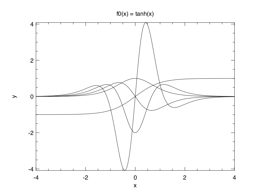
If you replace f0 in the previous example with the following definition, then you will have another good-looking figure :)
let f0 x = Maths.(
  let y = exp (neg x) in
  (F 1. - y) / (F 1. + y)
);;
As you see, you can just keep calling diff to get higher and higher-order derivatives. E.g., let g = f |> diff |> diff |> diff |> diff will give you the fourth derivative of f.
Example 2: Gradient Descent Algorithm
Gradient Descent (GD) is a popular numerical method for calculating the optimal value for a given function. Often you need to hand craft the derivative of your function f before plugging into gradient descendent algorithm. With Algodiff, derivation can be done easily. The following several lines of code define the skeleton of GD.
open Algodiff.D

let rec desc ?(eta=F 0.01) ?(eps=1e-6) f x =
  let g = (diff f) x in
  if (unpack_flt g) < eps then x
  else desc ~eta ~eps f Maths.(x - eta * g);;
Now let’s define a function we want to optimise, then plug it into desc function.
let f x = Maths.(sin x + cos x);;

let x_min = desc f (F 0.1);;
Because we started searching from 0., the desc function successfully found the local minimum at -2.35619175250552448. You can visually verify that by plotting it out.
let g x = sin x +. cos x in
Plot.plot_fun g (-5.) 5.;;
Example 3: Newton’s Algorithm
Newton’s method is a root-finding algorithm by successively searching for better approximation of the root. The Newton’s method converges faster than gradient descent. The following implementation calculates the exact hessian of f which in practice is very expensive operation.
open Algodiff.D

let rec newton ?(eta=F 0.01) ?(eps=1e-6) f x =
  let g, h = (gradhessian f) x in
  if (Maths.l2norm g |> unpack_flt) < eps then x
  else newton ~eta ~eps f Maths.(x - eta * g *@ (inv h));;
Now we can apply newton to find the extreme value of Maths.(cos x |> sum).
let _ =
  let f x = Maths.(cos x |> sum) in
  let y = newton f (Mat.uniform 1 2) in
  Mat.print y;;
Example 4: Backpropagation in Neural Network
Now let’s talk about the hyped neural network. Backpropagation is the core of all neural networks, actually it is just a special case of reverse mode AD. Therefore, we can write up the backpropagation algorithm from scratch easily with the help of Algodiff module.
let backprop nn eta x y =
  let t = tag () in
  Array.iter (fun l ->
    l.w <- make_reverse l.w t;
    l.b <- make_reverse l.b t;
  ) nn.layers;
  let loss = Maths.(cross_entropy y (run_network x nn) / (F (Mat.row_num y |> float_of_int))) in
  reverse_prop (F 1.) loss;
  Array.iter (fun l ->
    l.w <- Maths.((primal l.w) - (eta * (adjval l.w))) |> primal;
    l.b <- Maths.((primal l.b) - (eta * (adjval l.b))) |> primal;
  ) nn.layers;
  loss |> unpack_flt
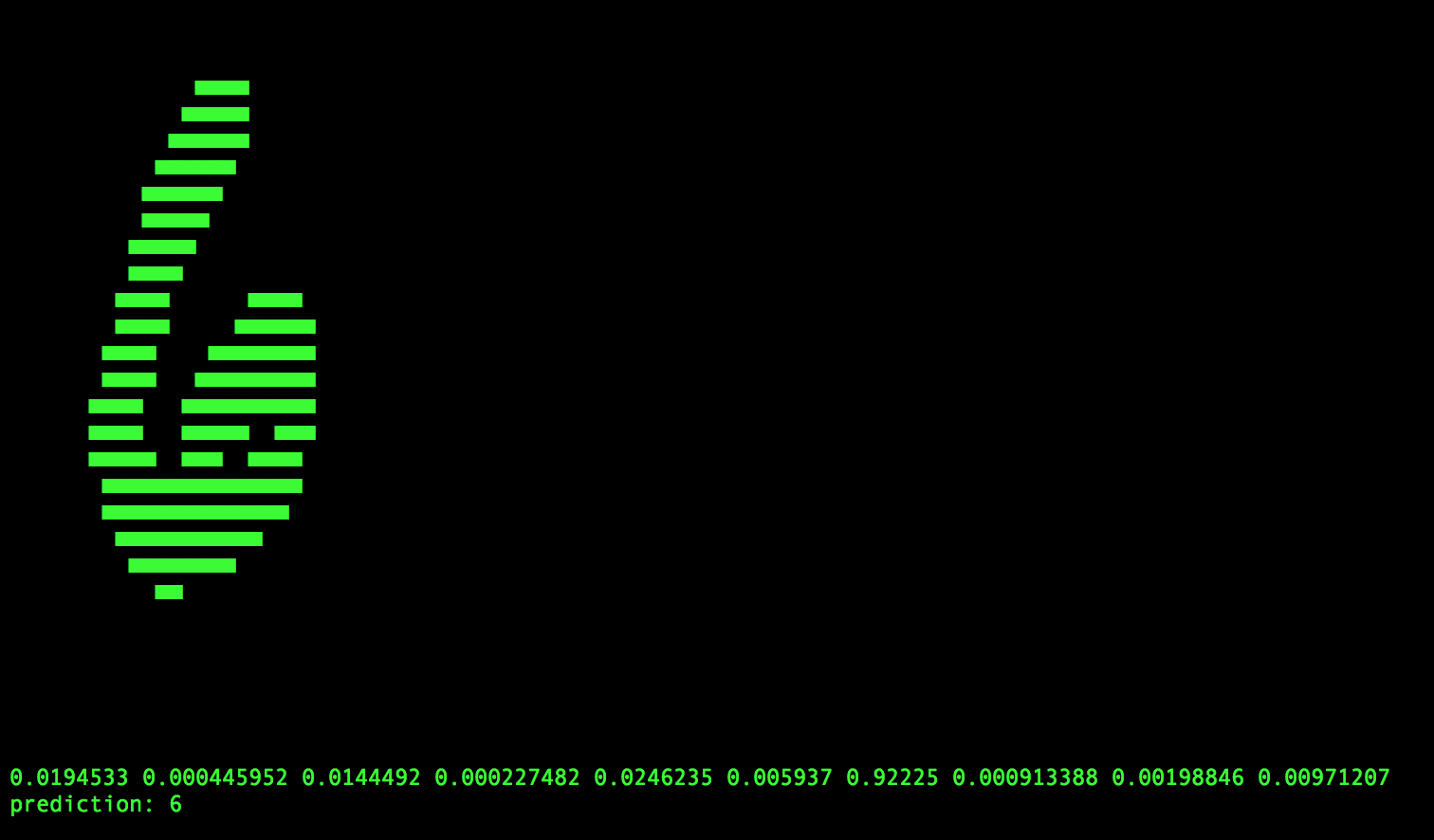
Yes, we just used only 13 lines of code to implement the backpropagation. Actually, with some extra coding, we can make a smart application to recognise handwritten digits. E.g., running the application will give you the following prediction on handwritten digit 6. The code has been included in Owl’s example and you can find the complete example in backprop.ml.
Example 5: Computation Graph of Simple Functions
Backward mode generates and maintains a computation graph in order to back propagate the error. The computation graph is very helpful in both debugging and understanding the characteristic of your numerical functions. Owl provides two functions to facilitate you in generating computation graphs.
val to_trace: t list -> string
(* print out the trace in human-readable format *)

val to_dot : tlist -> string
(* print out the computation graph in dot format *)
to_trace is useful when the graph is small and you can print it out on the terminal then observe it directly. to_dot is more useful when the graph grows bigger since you can use specialised visualisation tools to generate professional figures, such as Graphviz.
In the following, I will showcase several computation graphs. However, I will skip the details of how to generate these graphs since you can find out in the computation_graph.ml.
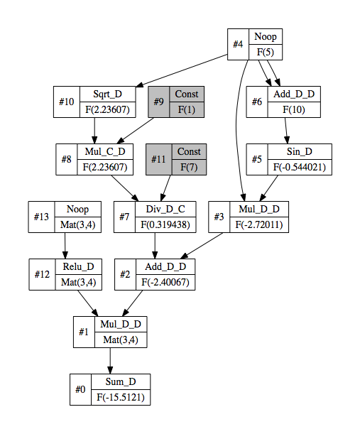
Let’s start with a simple function as below.
let f x y = Maths.((x * sin (x + x) + ( F 1. * sqrt x) / F 7.) * (relu y) |> sum)
The generated computation graph looks like this.
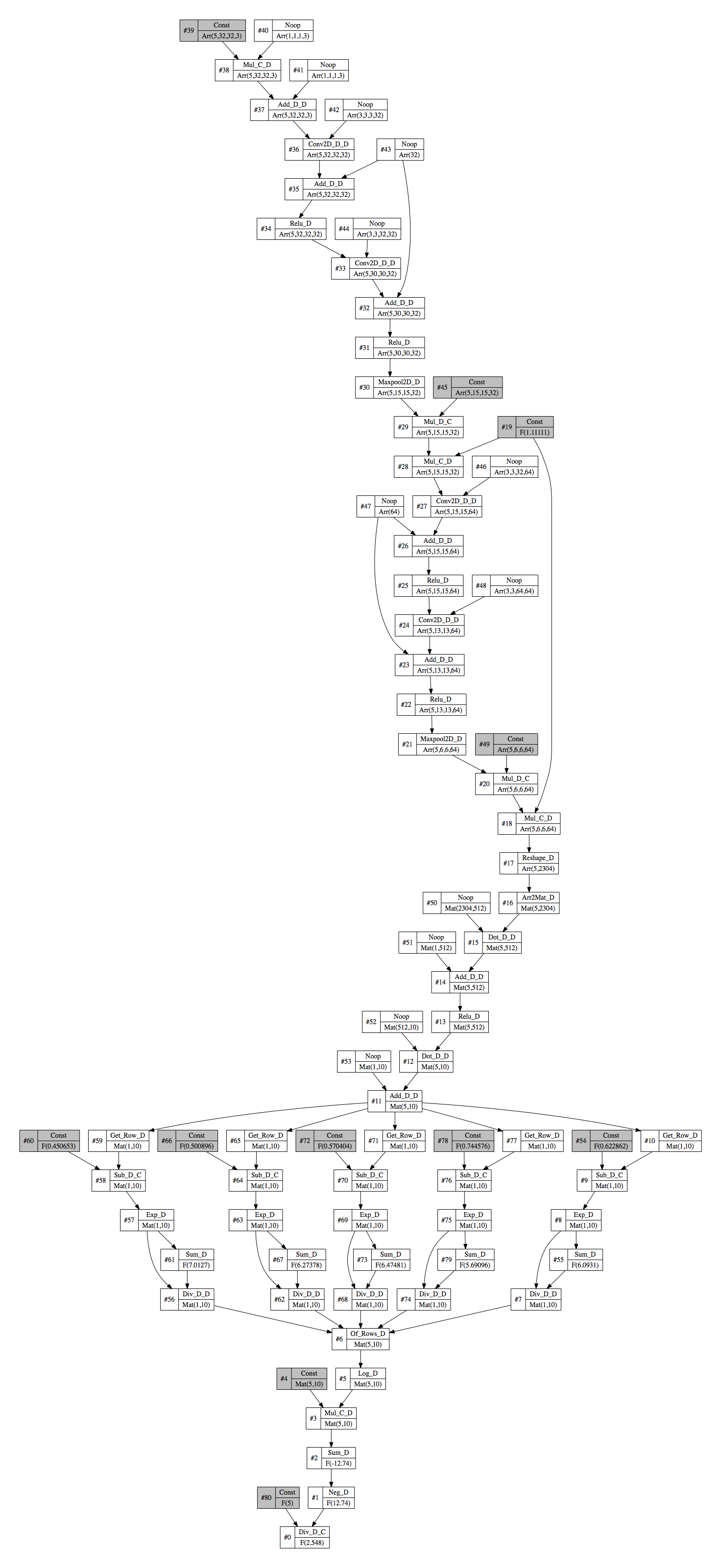
Example 6: Computation Graph of VGG-like Neural Network
Let’s define a VGG-like neural network as below.
open Neural.S
open Neural.S.Graph

let make_network input_shape =
  input input_shape
  |> normalisation ~decay:0.9
  |> conv2d [|3;3;3;32|] [|1;1|] ~act_typ:Activation.Relu
  |> conv2d [|3;3;32;32|] [|1;1|] ~act_typ:Activation.Relu ~padding:VALID
  |> max_pool2d [|2;2|] [|2;2|] ~padding:VALID
  |> dropout 0.1
  |> conv2d [|3;3;32;64|] [|1;1|] ~act_typ:Activation.Relu
  |> conv2d [|3;3;64;64|] [|1;1|] ~act_typ:Activation.Relu ~padding:VALID
  |> max_pool2d [|2;2|] [|2;2|] ~padding:VALID
  |> dropout 0.1
  |> fully_connected 512 ~act_typ:Activation.Relu
  |> linear 10 ~act_typ:Activation.Softmax
  |> get_network
The computation graph for this neural network become a bit more complicated now.
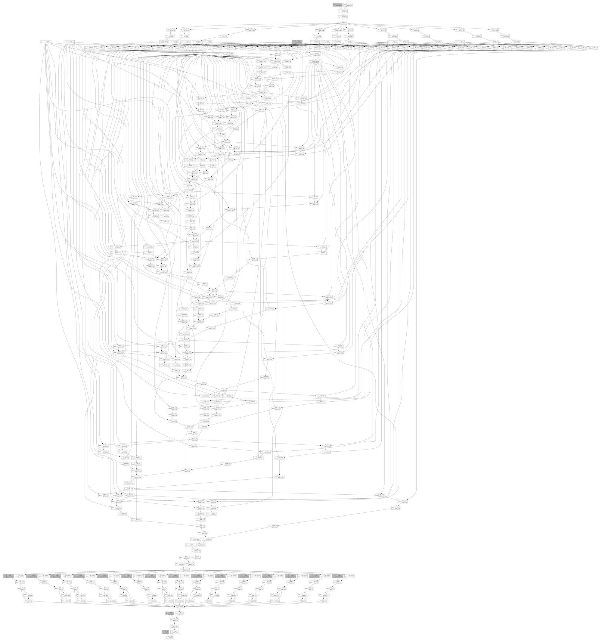
Example 7: Computation Graph of LSTM Network
How about LSTM network? The following definition seems much lighter than convolutional neural network in the previous example.
open Neural.S
open Neural.S.Graph

let make_network wndsz vocabsz =
  input [|wndsz|]
  |> embedding vocabsz 40
  |> lstm 128
  |> linear 512 ~act_typ:Activation.Relu
  |> linear vocabsz ~act_typ:Activation.Softmax
  |> get_network
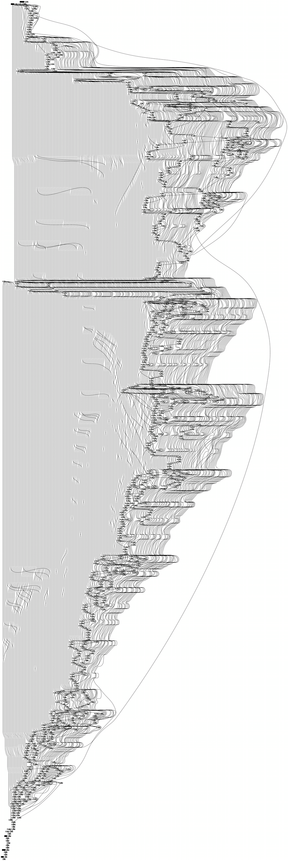
However, the generated computation graph is way more complicated due to LSTM’s internal recurrent structure. You can download the [PDF file 1] for better image quality.
Example 8: Computation Graph of Google’s Inception
If the computation graph above hasn’t scared you yet, here is another one generated from Google’s Inception network for image classification. I will not paste the code here since the definition of the network per se is already quite complicated. You can use Owl’s zoo system #zoo "6dfed11c521fb2cd286f2519fb88d3bf".
The image below is too small to check details, please download the [PDF file 2].