Definition

An Operating System (OS) is a piece of software which manages the computer’s hardware resources and moderates access to the hardware by all other pieces of software running on the computer. A modern OS is huge and does a lot of things, including:

• Abstracting hardware. So you can write programs that deal with generic inputs (e.g. a mouse) and not specific ones ( a Logitech mouse, a Microsoft mouse).

• Scheduling processes. Deciding which program gets to use the CPU at any given time. More about this shortly.

• Allocating Resources. Giving each running program its fair share of resources such as memory.

• Enforcing security. Putting in low level protection that limits the damage a rogue program can do.

• Providing a library of useful functions. This goes toward there being a platform as discussed in the “How Computers Work” primer. By providing a wealth of pre-defined functions, programs are easier to write, smaller and more uniform in look and behaviour.

Computer Eras

Computer architecture has transitioned through several eras. To illustrate the key ones, we’ll view a computer rather abstractly as a combination of users, applications (programs), operating systems and hardware. The first computing machines had no concept of an operating system and only ran one program so we can depict it as:

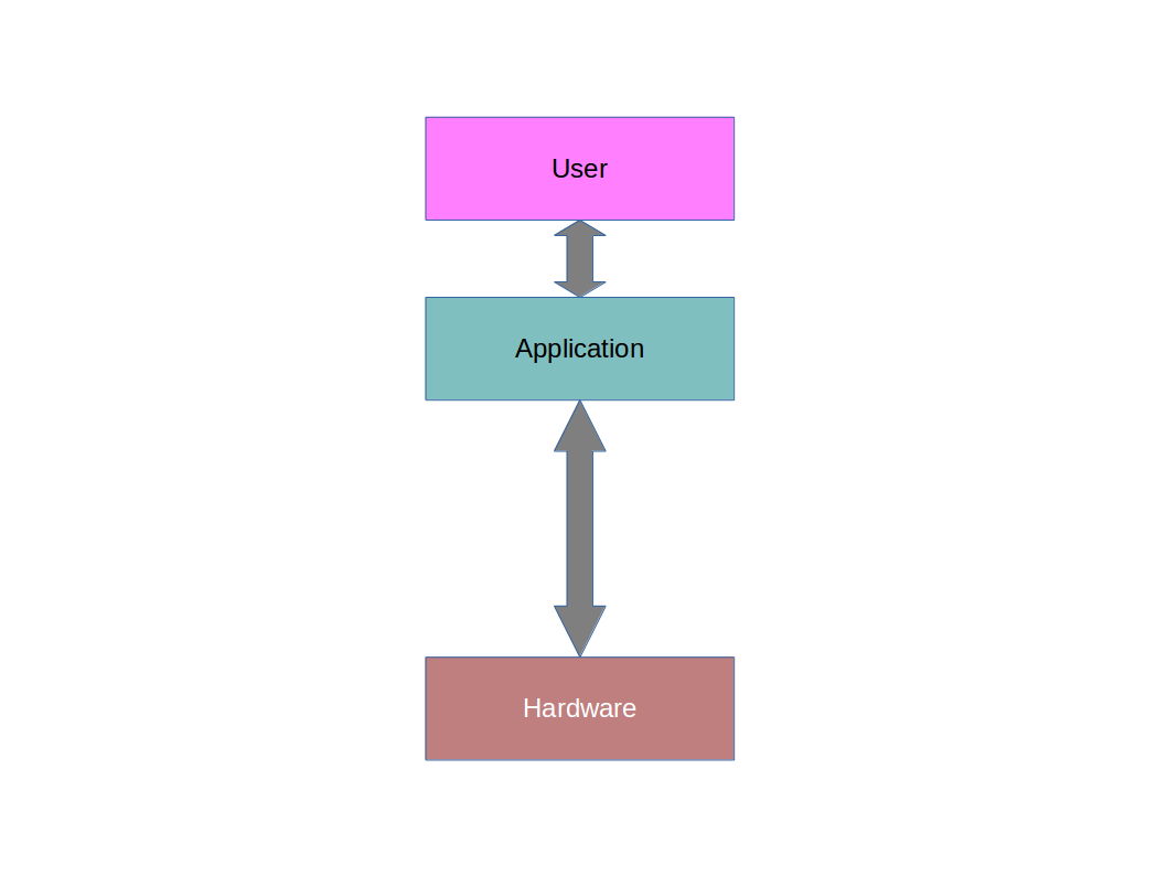
Here, there is one piece of hardware that runs a single program and is controlled by exactly one user.

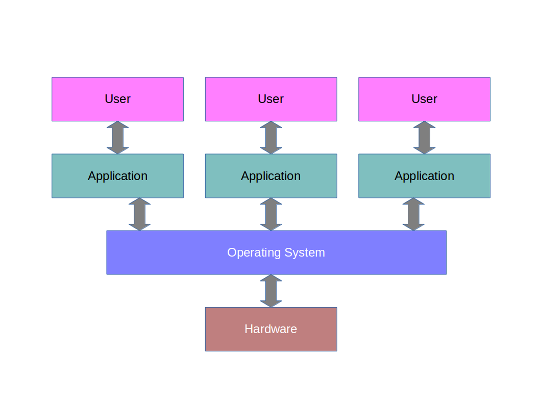
Then came the Time Sharing era. Here we had an enormous machine in the company basement and lots of dumb ‘terminals’ (screens and keyboards) connected to it, Each terminal did no processing itself - it just sent keypresses to the basement and received back data to display on the screen.

For this to work, the machine had to keep track of multiple programs (one per terminal), which it did with a rudimentary OS. This spoke to each terminal in turn, asking “do you have anything new to tell me?”, and pushing a screen update at the same time. When it wasn’t talking to a terminal, that terminal couldn’t update in any way. So it was a bit like holding ten telephone conversations at once, and skipping from one handset to the next, trying to keep all conversations going. Our abstract ‘architecture’ would look like:

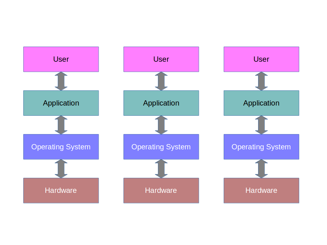
In the early 80s, the microprocessor era came about. The processing moved out of the basement and inside each terminal to make what we now call desktop computers. Initially these machines ran only one program at a time. Operating systems were used primarily to abstract away the hardware and allow for a method to load the program (you often had to load the program from some form of storage such as a cassette). The architecture diagram was then:

In the late 80s, the operating system became more important with the introduction of multitasking. The appearance of graphical interfaces (MS Windows etc) gave rise to the desire to run multiple programs at once and be able to switch between them. This gave rise this architecture:

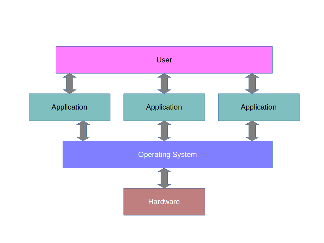
This is the era we will stop at for now since the following eras (of internet and mobility) lead to a significantly more complex picture.
It’s more useful for us to drill down on how the multitasking era was made possible.

Memory Protection

When a program is running on a computer it is called a process. A process on a modern operating system has no awareness of any other running process. This design ensures that one process cannot read or write to any memory used by another process, or the operating system itself. This is an important principle: a key aim of the operating system is to protect memory and prevent one process from affecting the execution of another.

At its simplest, the operating system allocates each process a specific chunk of memory (i.e. a range of addresses it can use). Accessing anything outside this range isn’t allowed (we need hardware support for this to make sure it can be enforced).

But how can you stop a process from using a different chunk of memory either inadvertently or intentionally? One way is to add an offset to any memory address a process requests. Let’s imagine the operating system gives our program the range 0x1200 to 0x12AA. If our program requests address 0x0001 the operating system steps in and adds 0x1200 so that the memory address becomes 0x1201. If it requests 0x1300 (just out of its range), the operating system spots this and terminates the process.

The nice thing about this is that the process is unaware of the offset added by the operating system, which means the programmer does not need to worry about the value of the offset with writing the program. It’s far from perfect however. How much memory should a given process get? Can we avoid wasting space by allocating memory to a process that either doesn’t need it at all or only needs it briefly? The answer is yes, and there are some clever schemes in operation to do these. Those who are doing Paper 2 (i.e. not the NSTs) will delve into this in the Operating Systems course.

Time-slicing and Scheduling

We know from our primer on hardware that that the multitasking architecture would require multiple Fetch-Execute cycles running simultaneously. Which effectively means one CPU per process, which even modern computers do not have. So how is this done? An operating system can borrow a trick from the old time sharing systems. In time sharing systems each terminal is given a small amount of time (a time slice or quantum) to each terminal. Similarly, a modern operating system can give each process a quantum of time on the CPU before moving onto the next in a round-robin fashion. So, consider programs (or processes) A, B and C running on a machine, and then D gets started:

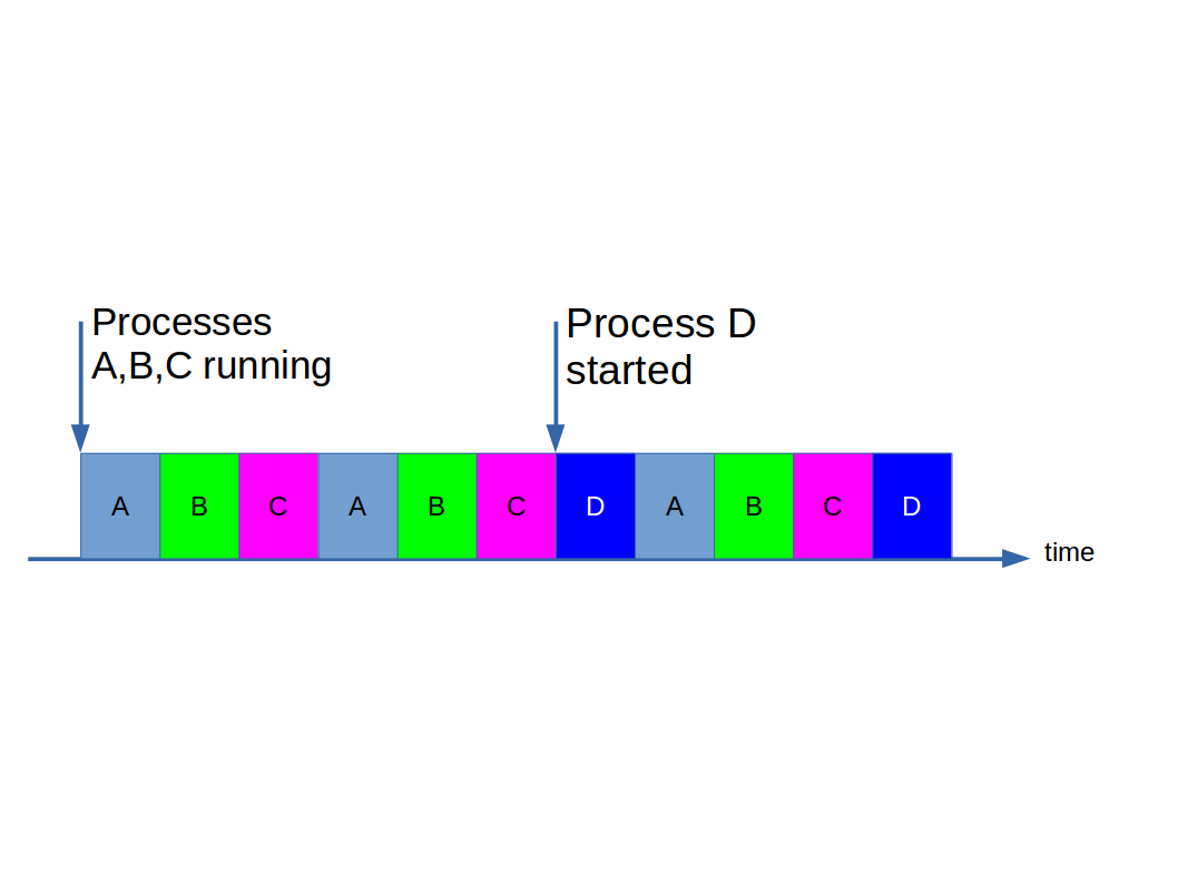
The idea exploits the high speed of the fetch-execute cycle compared to the update rate of our senses (eyes in particular). If we keep that timeslice really short (milliseconds) then the brain is fooled into thinking everything is running at the same time when in fact it is not. We call the component of the operating system that controls the switching (when it occurs and which process goes next) a scheduler.

Of course, switching from one program to another is non-trivial. A running program has a lot of CPU state associated with it, such as register values, the IB value, the PC value, etc. The CPU must stop what it is doing, copy all this state to somewhere in main memory, load in all the state for the next process from main memory and then start where it left off on that process. This is called a context switch and understandably it takes a bit of time.

We choose the time slice based on balancing our desire to switch tasks very frequently (to give a better impression of programs running simultaneously and make the system feel responsive) with the desire to minimise the number of wasteful context switches we have to do:

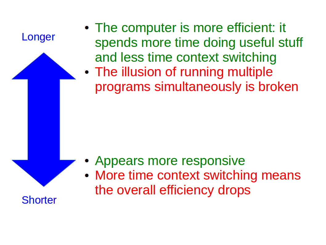
The exact choice is more an art than a science, but it’s 20ms to 100ms on most operating systems today.

Blocking and Interrupts

Whilst a few tens of milliseconds sounds like a short time to us, it’s an age to a computer. Sometimes a process can do all it can do before its time slice expires. For example, it might make a request to load some data from a hard disc, or decide to wait for a keypress before proceeding. When a process has not finished but is stuck waiting for something else to happen, we say it is blocked. It can yield the remainder of its time slice if it’s being good:

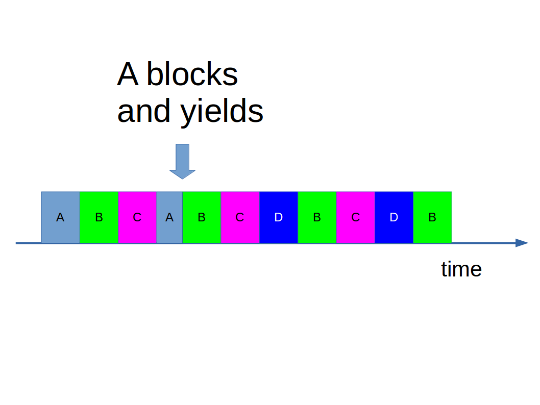
We obviously don’t want to keep giving a blocked process time slices until it is unblocked and can do something with them. So when a process is blocked, the scheduler takes it out of the running process queue as illustrated above.

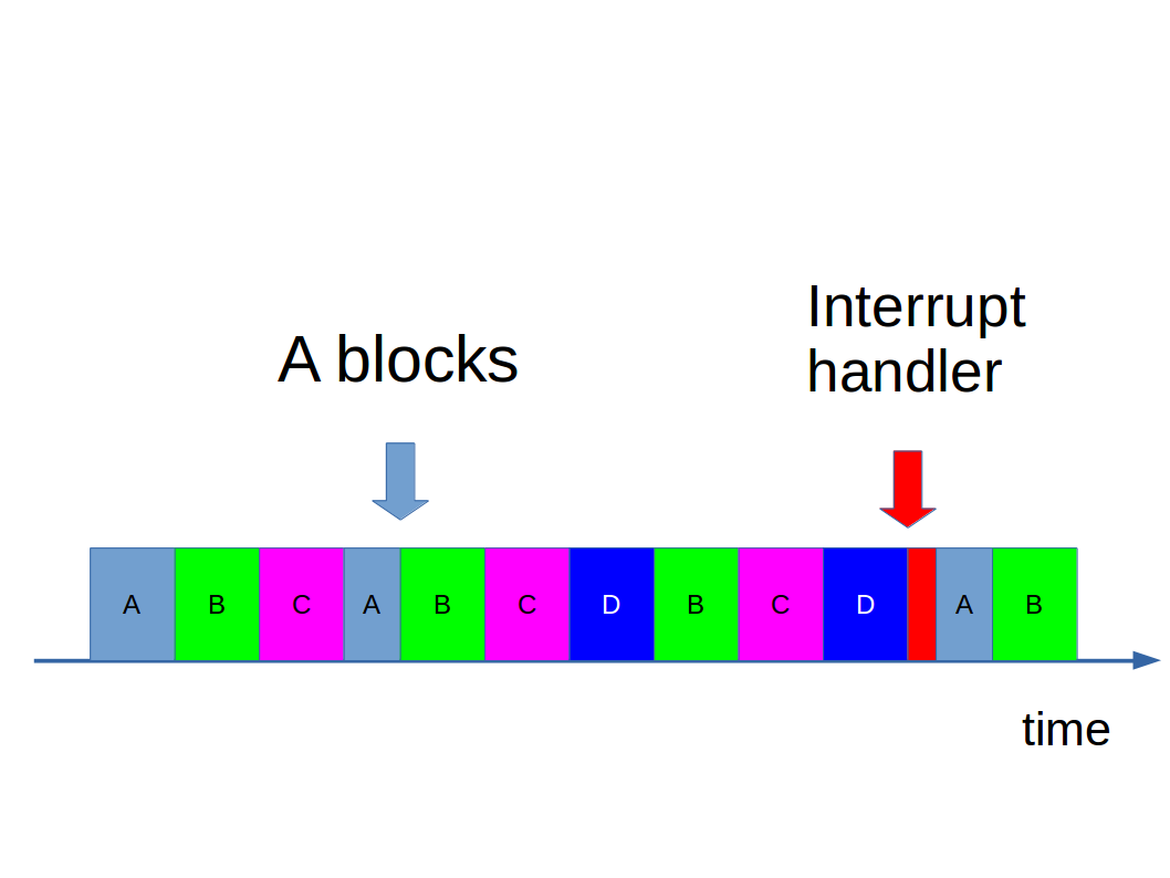
Now we are faced with the problem of knowing when to reinsert it into the running queue. We could poll it, by which we mean periodically check to see whether it is ready to be unblocked. This works fine, but rather limits performance (you have to keep checking, which doesn’t come for free).

Instead CPUs feature interrupts. These are a special communication path between the CPU and peripherals such as the hard disc. When the peripheral has finished doing whatever it was asked to do, it sends a signal along this wire to tell the CPU that the wait is over. We call this raising an interrupt and it’s obviously a lot more efficient than polling. The operating system runs an interrupt handler which sticks the process back in the running queue on the scheduler.

In this way we get efficient use of the CPU and a responsive machine.

Threads and Concurrency

Sometimes a program needs to do background tasks while still performing something in the foreground. This is easy to see for a graphical application, for example. It might be running an intensive computation but still wants to process mouse clicks to allow a cancel button. For this we have threads. These are sub-processes of a process that are scheduled independently:

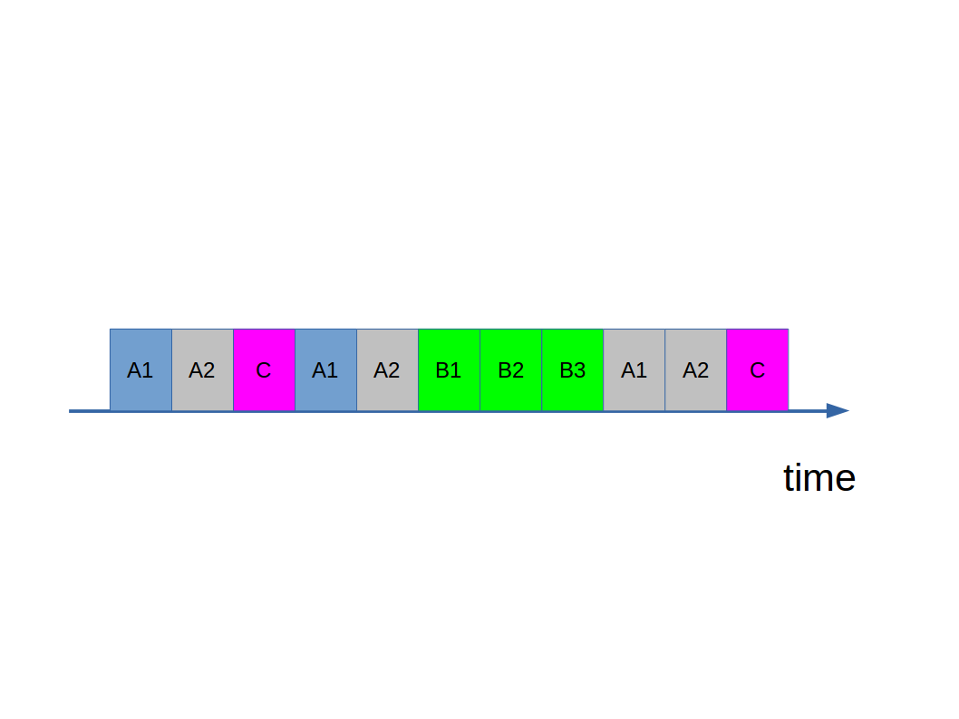
Here process A has two threads (A1, A2) and B has three (B1, B2, B3). Each thread within a process runs independently (has a separate Fetch-Execute cycle) but shares the main memory with other threads in the process*:

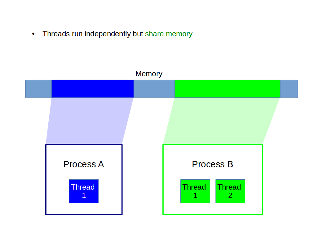
This is very useful: the threads can share data just by writing to the shared memory. But it adds a new complication: concurrency. The complexity is so significant that we avoid working with threads this year wherever possible, Those who stick around for IB Computer Science will study concurrency in great detail. Here it is just good for us to understand what might go wrong.

Race Conditions

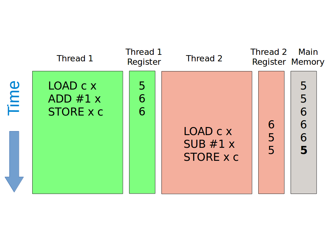
Consider a value 5 stored in main memory and two threads that wish to write to it. One thread adds one, the other subtracts one. In simple code terms:

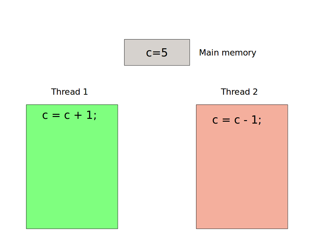
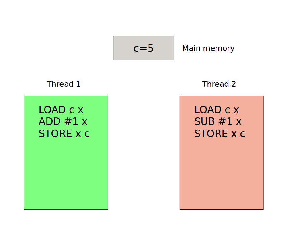
This boils down to some simple (pseudo) assembly/machine code:

Let’s now consider what happens when these threads run concurrently. One possibility is that thread 1 gets a time slice and does everything in that slice. This means the value in main memory will be 6 at the end of the slice. Then thread 2 runs and we end up with the value 5 in memory:

But what if there is a context switch at an inopportune moment? Perhaps thread 1 will get to run its first instruction but then thread 2 jumps in:

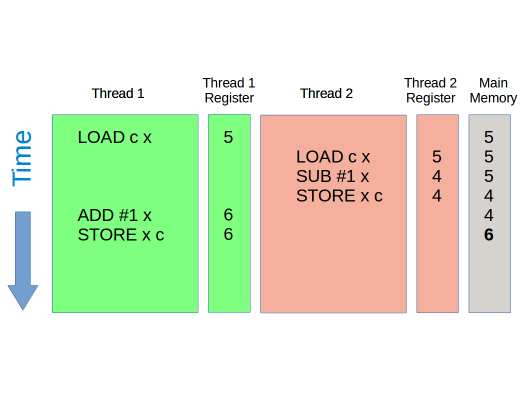
Here we see that thread one looks in memory and copies the value 5 to a register. Thread 2 jumps in and copies the same value (5) to its register. Thread 2 subtracts one and updates the main memory to 4. But then thread 1 completes its task, based on the value it copied into is register (which was 5 not 4). It adds one and thus stores 6 to main memory.

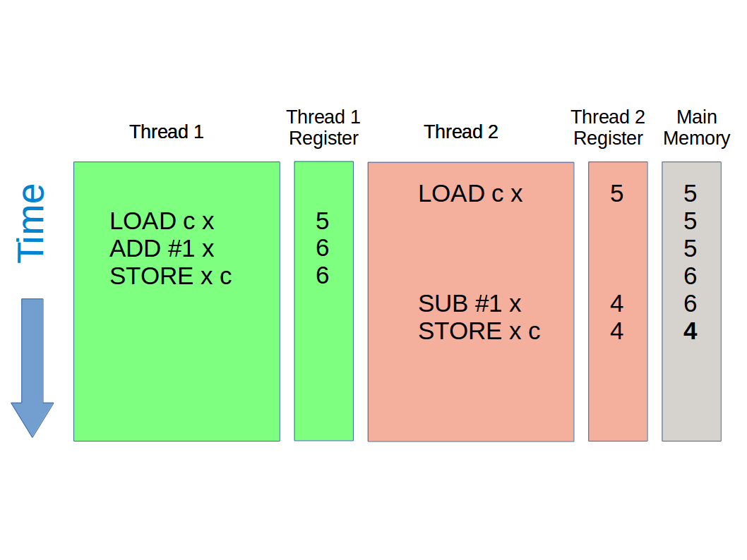
The inverse of this is equally possible, and results in the value 4 in main memory.

So here we have one program with (at least) three possible results. As a programmer we have no way of knowing which we would get. In fact, it’s non-deterministic (i.e. could give different answers if you repeatedly run it). This is called a race condition (the output depends on which thread does what first).

We’re not going to solve it here: all you need to understand is that concurrency introduces nasty complexities like this. Hence we avoid threads and concurrency this year.

Immutability

You’ll hear a lot about making data immutable this year. Immutable data is initialised to some value and can never be changed. At first this sounds silly: programs are all about manipulating data and now we’ll have to waste resources making new values rather than changing established ones.

In fact, there are various advantages to immutable data. One of the key ones is that you can’t end up with race conditions and so writing thread-safe code is much simpler.

Conclusion

Operating Systems are an integral part modern computers. They are extremely complex pieces of software that manage all the computer resources. They allow for multitasking and threading, the latter of which introduces new layers of complexity such as race conditions.