How Computers Work
This document is a simple introduction to the fundamental principles of a computer. (c) Dr Robert Harle, 2015.
A ‘Notebook’ Computer
We’ll start our exploration of how a computer works by looking at some of Alan Turing’s work. In 1936 he described a theoretical machine that could be used for ‘computing’, a so-called Turing machine. Although not what we would think of as a computer today, the core principles are the same and they can be presented without worrying about specific technologies, which is very useful for this overview.
The original machine envisaged reels of paper that were divided into cells that could be written to. The theoretical construct assumed the reels were infinitely long so you never have to deal with running out of paper. I’d strongly encourage you to take a look at the excellent website http://aturingmachine.com, which has an actual implementation of a Turing machine (albeit not one with an infinitely long reel!).
Our setup will be slightly different, but only in the details. We will have an empty notebook, two pieces of paper, a pencil and an eraser. These are all easily obtained so you can make the ‘computer’ if you feel keen. Following through the steps in some form is very important though. If nothing else, if you enjoy the sort of puzzle that writing ‘programs’ for our pseudo-computer entails, you can be confident computer science is a good choice for you!
The Rules
Now for some rules. Each page in the notebook can be empty or contain the number zero or the number one. There are only a few actions you’re allowed to take, and we label them with some shorthand:
| Symbol | Meaning |
|---|---|
| + | Go forward one page in the notebook |
| - | Go backward one page in the notebook |
| W0 | Delete anything on the page and write a zero |
| W1 | Delete anything on the page and write a one |
| D | Delete anything on the page |
| R | Read the symbol on the page, which may be 0, 1, E (empty page), or X (representing the front or back cover). |
The Action Table
One of our two pieces of paper will contain the “action table”, which represents the program that the computer executes. It can be drawn out as a table as follows:
| Read | Actions |
|---|---|
| 0 | W1, + |
| 1 | + |
| E | W1, + |
This table is just a set of simple rules: if you read the symbol in the first column then carry out the actions in the second column. So, if we start with the first page of a blank notebook, it will read E (empty) and so write a 1 on the page (W1) and move forward to the next page (+). Crucially, it then repeats.
So this rather silly program will just write a one on every page in the notebook. (There’s clearly a problem when we reach the end of the notebook, but let’s ignore that for now!).
Adding Global State
If you play around with what we have so far, you’ll find this action table is pretty limiting. We don’t, for example, have a way to say “write only ones on the first two pages”. We fix that by creating multiple sets of actions for the same input. In order to decide which set to run, we need the system to have a simple ‘state’, which in our case will be a letter (A,B,C,..) on the second piece of paper. We’ll have a special state (label it ‘H’ for halt) that causes our program to terminate.
Now, we also need to extend our action table:
| State | Read | Actions | Next State |
|---|---|---|---|
| A | 0 | W1, + | B |
| A | 1 | + | B |
| A | E | W1, + | B |
| B | 0 | W1 | H |
| B | 1 | H | |
| B | E | W1 | H |
What does this do? Starting with the first page (assumed empty) and in state A we first follow this line:
| State | Read | Actions | Next State |
|---|---|---|---|
| A | E | W1, + | B |
And so we write 1 on the first page, move forward one page and update the state to B. Now we read another empty page but we’re in state B so we follow this line:
| State | Read | Actions | Next State |
|---|---|---|---|
| B | E | W1 | H |
Which writes a 1 and ends the program (state H). The result is that it wrote ones to the first two pages (only).
A More Interesting Program
Let’s develop the equivalent of the counting program you can find at the aturingmachine.com site:

Our version will start with an empty notebook and count in binary, overwriting any previous number with its successor. For example, if the notebook currently contains the value 7 in binary, then after the action table instructions have been followed the value 8 in binary will be written in the notebook. To do this, you obviously need to understand how binary addition works. If you don’t, then you should look at the other mini-course in this series on Bits, Bytes and Number Systems before proceeding.
We’ll need four states: States A and A’ will initialise the last page to 1. State B will move through the notebook until we find the last non-blank cell in the notebook. State C will handle the adding and carrying of bits. State A is very easy to define:
| State | Read | Actions | Next State |
|---|---|---|---|
| A | E | + | A |
| A | X | - | A’ |
| A’ | E | W1 | B |
This moves us through the notebook until we find the back cover, then moves us one page back, writes a 1 and moves to state B.
State B is the start of our main cycle. It moves forward through the notebook until it finds the (back) cover, then it goes back one page and moves into state C. So we have:
| State | Read | Actions | Next State |
|---|---|---|---|
| B | 0 | + | B |
| B | 1 | + | B |
| B | X | - | C |
State C is the only clever bit. When we move into it we’ll be looking at the last page thanks to state B. So we know we’re looking at the Least Significant Bit (LSB) of the binary number. If it’s a zero, we just change it to a one and we’re done with this number and the cycle starts again with state B:
| State | Read | Actions | Next State |
|---|---|---|---|
| C | 0 | W1 | B |
If it’s a one, we turn it to a zero and repeat state C starting on the previous page (in effect we carry the bit to the left). We are done with this number when we find a zero, or we find an empty page, or we get to the front cover. So:
| State | Read | Actions | Next State |
|---|---|---|---|
| C | 1 | W0, - | C |
| C | E | W1 | B |
| C | X | H |
Now, if it was a 0, we have just changed it to a 1 and there is no carry so we are done. We can move onto the next integer by switching back to state B:
| State | Read | Actions | Next State |
|---|---|---|---|
| C | 0 | W1 | B |
Putting all that together we get:
| State | Read | Actions | Next State |
|---|---|---|---|
| A | E | + | A |
| A | X | - | A’ |
| A’ | E | W1 | B |
| B | 0 | + | B |
| B | 1 | + | B |
| B | X | - | C |
| C | 0 | W1 | B |
| C | 1 | W0, - | C |
| C | E | W1 | B |
| C | X | H |
If you find this all quite easy, it’s a useful exercise to wrtie some of your own ‘programs’ for this system. As optional challenges:
Can you write a version of the counting program so the MSB of the number is always on the first page (i.e. not start at the last page)?
Can you write a program to countdown from ten (you’ll need to initialise it to ten and implement subtraction! This is quite hard)?
Adding More State
Let’s try to modify our counting program so that it counts from 1 to 3 and then ends. Our challenge is to recognise when we are at 3, which we’ll have to do by somehow tracking where we’re at. With the tools we have there are two possibilities:
Give every integer its own set of states in the action table. So, instead of returning to state B after the first time we have finished state C, we move to a state D. This new state is a clone of the rules for state B, except that it moves to state E not C. The fact we are in state D implies that we are currently moving from 2 to 3. This method works, but the action table is lengthy and confusing (imagine how many states we would need if we wanted to stop at 32!).
Check all the pages every time we are about to move on to the next integer (which is whenever we transition from state C to B). We would need an extra set of states that walks through the integer in the notebook and checks whether it matches 3. If it does, stop. If not, back to state B, and keep going.
Neither approach is quite satisfactory, although both work. In terms of efficiency we would rather expand our global state to keep track of the number we’re on. This would involve a new column (to handle changes to the new piece of state) but overall adding more state will make our program easier to code and faster to run.
Moving to a Modern Computer
Obviously a modern computer doesn’t contain a notebook, but it can be seen as an advanced implementation of our ‘machine’. We can map the key components pretty easily:
The action table becomes the program, stored somehow.
The notebook is the data, which is stored in electronic memory
The state is internal data, which differs from normal data since anyone using the program is unaware it exists. It is still stored in electronic memory though.
The interpretation of the action table (by a human) becomes the interpretation of the program, which is done by the Central Processing Unit (CPU)
Memory
For this course we don’t need to delve into the gory details of computer memory technology, but it is useful to have a high-level idea of how it works. Computer memory is a very large collection of memory cells, which are just small electronic circuits that can store a single bit (i.e. 0 or 1). There are various types of memory cell available, but we generally look for the fewest components possible (cheaper and smaller).
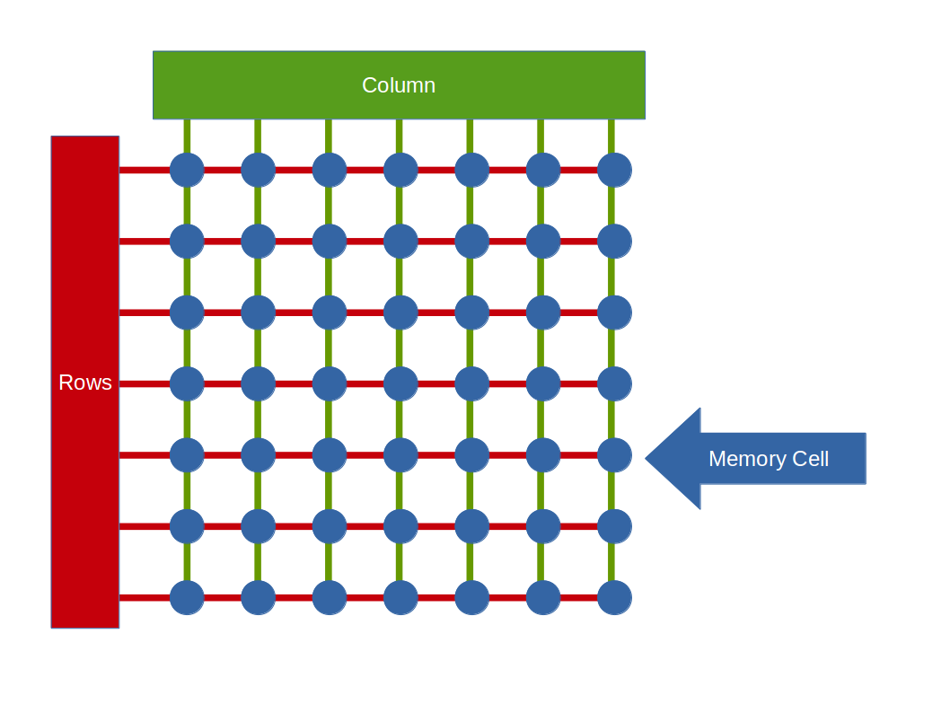
The cells are usually arranged in a grid like this. The idea is that a specific bit can be read or written by first selecting a row and then a column using electronic switches (transistors). The interesting thing about this is that it takes the same time to access the first cell as the last one. We have what we call Random Access Memory (RAM) since we can randomly jump around reading data without a latency penalty (alternatives to RAM are discussed at the end of this section). You will likely come across two types of RAM cells: DRAM and SRAM (others do exist but these two are dominant):
Dynamic RAM (DRAM). A DRAM cell is basically a capacitor and a transistor. You may recall from physics lessons that a capacitor can be used to store charge: you pump it in, then you can take it out when you want. This makes it an obvious choice: we can use a discharged capacitor to represent a ‘0’ and a charged capacitor a ‘1’. The transistor is just a switch that selects the charge or discharge mode. Simple, cheap and space-efficient. But there’s a problem: charged capacitors naturally leak charge over time. So 1s eventually become 0s! To fix this you need to regularly stop all memory accesses, and look at each capacitor to decide whether its charge needs to be topped up or not. This refresh cycle has to occur hundreds of times each second and, while it’s happening, the DRAM is essentially useless. This refresh operation is handled inside the memory chip itself.
Static RAM (SRAM). An SRAM cell is a collection of four to six transistors forming what is called a bi-stable circuit. This solution has the advantage of faster read and write times, but the extra components are expensive and make the cells rather large (limiting capacity when compared to DRAM).
In practice, the 16GB or so of memory that our computers come with is almost entirely DRAM. The cheaper, smaller cells keep costs down so, for a given amount of money, you can buy more RAM. There is a performance penalty associated with constantly having to refresh, but in modern DRAM implementations this is not significant.
That said, there are parts of a computer where we just can’t be waiting for DRAM operations to complete. So we use small chunks of SRAM (MB not GB) wherever we need really fast performance (e.g. within the CPU as you’ll see).
One more thing on memory before we move on. We know that if nothing refreshes a cell, the information is eventually lost. So data only survives while the computer is powered on and hence able to refresh the cells. We call this volatile memory (power off, data lost). We therefore need some form of non-volatile memory (power off, data intact) to store things between power cycles. For today’s computers that means a hard disc, which you get in one of two flavours:
HDD. A traditional Hard Disc Drive has a spinning platter with lots of tiny magnetic ‘pits’ on it. There is a read and a write head (think CD player on steroids) that can measure or change the magnetic state of the pit beneath it as the platter spins. This is a form of Sequential Access Memory (SAM) since we can’t just jump randomly to a pit: we have to wait until it comes round on the platter. HDDs offer an excellent capacity-to-cost ratio. However, they are painfully slow compared to RAM.
SSD. A Solid State Disc (SSD) uses the same core technology as USB sticks to store data without power. The physics behind them is rather complex and beyond scope here. The key points are they’re not cheap and they don’t quite have the performance of RAM, but they are random access and still much faster than a HDD. Costs seem to be falling fast at the moment as data capacities increase.
The CPU
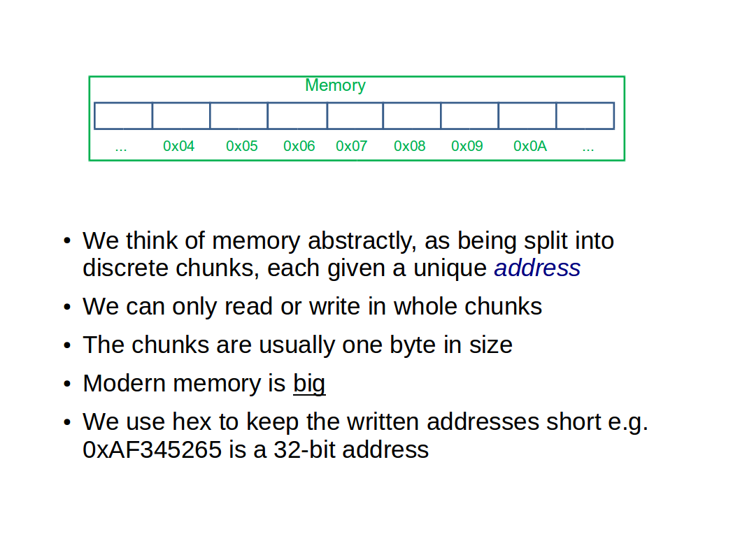
We’ll use a (highly simplified) model of a computer as illustrated above. It contains three hardware components: a Central Processing Unit (CPU), some main memory (DRAM), and something to interconnect the two (a motherboard). Although we’ve just delved into the innards of the memory, all we care about here is that there are a number of memory `slots’, each a byte in size, and each addressable through some unique number:
The CPU is really a collection of electronic circuits that includes:
A register bank. Small chunks of super-fast SRAM memory embedded in the CPU to store internal data/state being worked on. We might have just tens of registers, each of size 64 bits (yes, just bits).
An Instruction Buffer (IB). A special register that holds a copy of the current instruction (action table rule) we are dealing with.
A Program Counter (PC). A special register that holds the memory address of the next instruction to be processed.
A Memory Access Unit (MAU). A piece of electronics that shifts data back and forth between main memory (DRAM) and the registers. A CPU can only act on values in registers.
An Arithmetic Logic Unit (ALU). A piece of electronics that can read integer values from the registers and perform arithmetic (addition, multiplication, etc.) on them, storing the result back in another register.
A Branching Unit (BU). Some electronics that allows us to execute conditional behaviour (e.g. if A then B else C). We’ll come back to this.
The last three in that list are known as functional units of the CPU. A modern CPU has many functional units, each carrying out a specialised task such as the ones above.
How much Memory can we use?
A consequence of this CPU structure is that the PC register (the one that contains the memory address of the next instruction) is of finite size. What this means is that there are only a finite number of memory slots that a given processor can support.
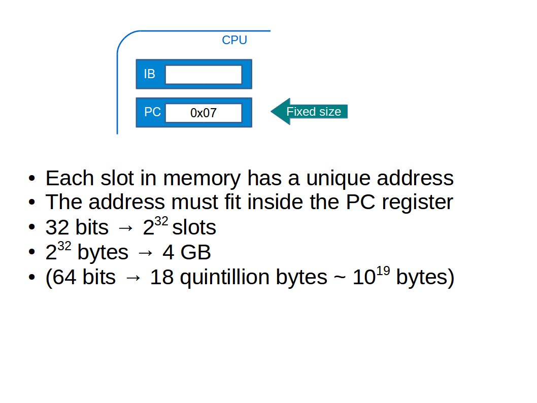
Rewind around 10 years and CPUs were mostly 32-bit (i.e. their registers were 32 bits long). So you simply couldn’t use more than 4GB of memory. So we moved to 64 bits. Which is more than anyone could ever need…err, right? ;-)
The Program
Just like our action table was a collection of rules, our program is a collection of instructions. Each instruction addresses a functional unit within the CPU, telling it to do some thing. We’ll create a few very simple instructions our CPU can understand:
| Instruction | Meaning |
|---|---|
| L-X-R | Load the data at main memory address X into register R |
| S-R-X | Store the data in register R in main memory at address X |
| A-X-Y-Z | Add the values in registers X and Y and put the result in register Z |
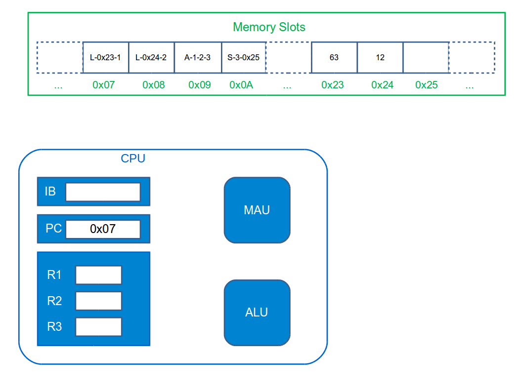
Note that this means we have to do four instructions just to add two numbers currently in memory (say, at address 0x23 and 0x24):
L-0x23-1 # Load first value (currently at memory slot 0x23) into register 1
L-0x24-2 # Load second value (currently at memory slot 0x24) into register 2
A-1-2-3 # Add the values and store the result in register 3
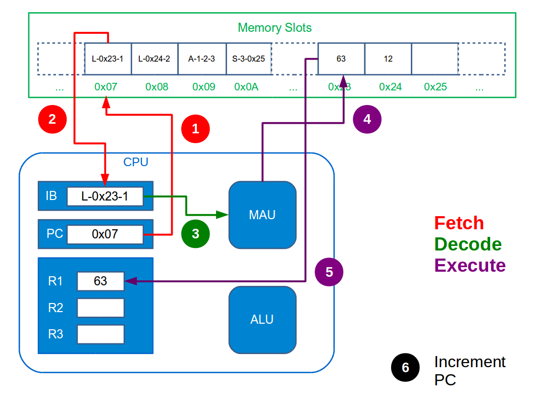
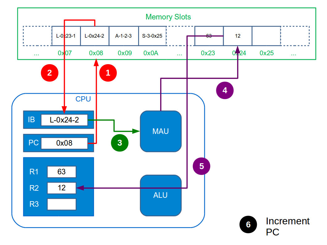
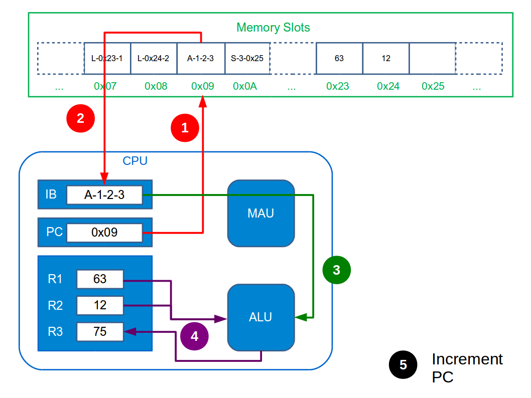
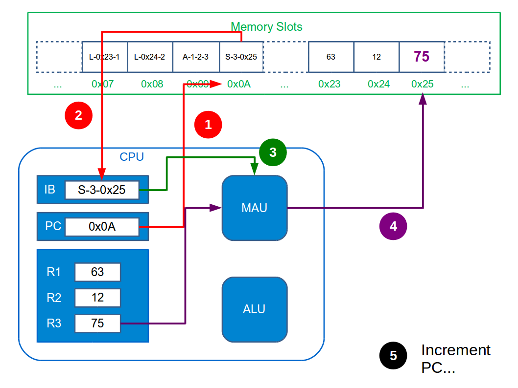
S-3-0x25 # Store the answer in register 3 in main memory (slot 0x25)The Fetch-Execute Cycle
The Fetch-Execute (or Fetch-Decode-Execute) cycle is the name given to what the CPU does. It maps directly to what you were doing when you worked through the notebook example: you figured out which line of the action table to read, then deciphered it and made any changes necessary, before repeating that process. Here it breaks down to:
Fetch the next instruction from main memory. This involves feeding the MAU with the memory address in the Program Counter and telling it to store it in the Instruction Buffer. After doing this the Program Counter is incremented.
Decode the instruction in the Instruction Buffer. This just means figuring out which functional unit to send it to and doing so.
Execute the instruction within the chosen functional unit.
The CPU just does this cycle over and over forever. Incrementing the Program Counter ensures we don’t just execute the same instruction forever. The figure below illustrates the whole tedious process necessary just to add two integers.
You’re probably aware that CPUs have frequencies associated with them—e.g. Intel i7 3GHz. This is the frequency at which the CPU can complete cycles. So a 3GHz machine can do 3,000,000,000 cycles (=instructions) a second! Really it’s not what computers can do, but how fast they can do it that is impressive.
Where is the program stored?
Note that the figures above show the program shoved somewhere in the same memory as the data (i.e. the numbers 63, 12, and 75). This makes our main memory a jumbled interleaving of code (instructions) and data.
This is an interesting choice that has some quite serious consequences. In particular, it allows for a program to write data into a slot containing an instruction, thereby wiping out that part of the program. This might be accidental (in which case the program will crash when it gets to that memory slot and tries to treat it as an instruction) or deliberate.
Conditional Execution
So far we’ve avoided dealing with conditional execution. We’ve just assumed that the Program Counter increments with each cycle. If that were true we could only ever move through a program sequentially and it would not be able to adapt its behaviour based on the data being fed in. In reality, we need this functionality and it’s supported by another functional unit: the Branching Unit. This unit is able to update the Program Counter and so allows us to jump around in a program.
To understand how it works we’ll add some new instructions to our imaginary CPU.
| Instruction | Meaning |
|---|---|
| B-P-A-B | If register P is not zero, update the PC to A, else update it to B |
| B-P-Q-A-B | If register P is greater than register Q, update the PC to A, else update it to B |
Here’s an adapted version of our previous program. Here each line is prefixed with an imaginary address for the instruction
0x77  L-0x23-1         # Load first value (currently at memory slot 0x23) into register 1
0x78  L-0x24-2         # Load second value (currently at memory slot 0x24) into register 2
0x79  L-0x25-3         # Load third value (currently at memory slot 0x25) into register 3
0x7A  B-1-0x7B-0x7E    # If register 1's value is > 0 then go to 0x7B else 0x7E
0x7B  A 1-2-4          # Add the values in registers 1 and 2 and store in 4
0x7C  S-4-0x26         # Store the answer in register 4 in main memory (slot 0x26)
0x7D  H                # Halt
0x7E  A 2-3-4          # Add the values in registers 2 and 3 and stores in 4
0x7F  S-4-0x26         # Store the answer in register 4 in main memory (slot 0x26)
0x80  H                # Halt
This program loads in three integers from main memory. If the first one is greater than zero, it adds values 1 and 2, puts the result in 4, stores 4 to main memory and finishes. However, if the first value is zero, it instead jumps to memory slot 0x7E, which leads it to add registers 2 and 3.
Machine Code
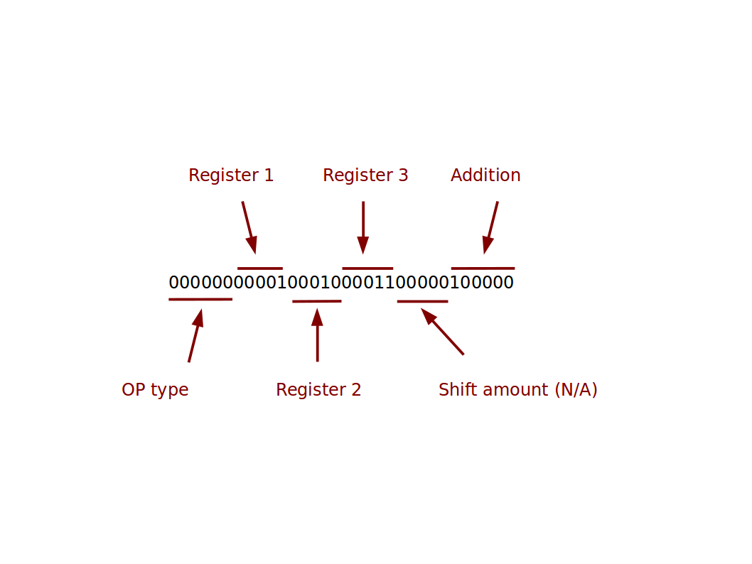
We have considered a very generic, simplified CPU with a very limit set of instructions. A real instruction is a binary number that can be stored in the instruction buffer (and so is limited in size to the instruction buffer). Here’s an example for a MIPS processor:
A program is just a sequence of instructions in a form understood by the processor. We call this form machine code. It’s perfect for a computer, but very hard for a human to work with.
Assembly Code
Our simple instruction language was more human readable (e.g L-0x23-1). Assembly code is the equivalent of this for a real CPU. It allows humans to write more meaningful text that translates directly to machine code. For example in MIPS:
   lw     $t0, 4($gp)       # Load value (n) at address 4 in main memory ($gp) into register $t0
   addi   $t0, $t0, 3       # Add 3 to the value (n=n+3)
   mult   $t0, $t0, $t0     # Square the value (n=n*n)
   sw     $t0, 0($gp)       # Store the answer back in main memory, address 0
will translate to four binary instructions. Programming involves writing assembly code like this (or worse) and you need to know about the instructions supported by the CPU. In some cases, writing in assembly language is the only way to obtain the performance required. However, the Cambridge course does not focus on programming in assembly since other programming languages provide a better environment in most cases (quicker development times, lots of useful existing libraries of code, better support for finding errors, and so on). For now just need to know what assembly code is, and how it relates to machine code.
CISC and RISC
As CPU designs were improved, it was tempting to add more complex, compound instructions to a CPU. For example, why not have one operation that did the entire addition program we had previously in one instruction—we might write A-0x23-0x24-0x25 for example. This is easier to work with and faster (it allows the CPU to potentially do the addition in one cycle not four).
This sounds like a good idea, but presents some issues. Firstly, our set of instructions becomes huge, making the job of assembly programming or compiler writing harder. Secondly, we’ll need more electronics to handle the new instructions (costs more and results in bigger and hotter chips). Finally the instructions themselves become much bigger. But that potential for a performance boost is tempting…
Too tempting for Intel and many of its competitors, who committed early on to this idea of a large set of complex instructions to eek out speed—called Complex Instruction Set Computing (CISC). They defined a particular instruction set, called x86, that is the core instruction set a computer must implement to run “PC” software. If you’re really keen, you can see all x86 instructions online.
The alternative is Reduced Instruction Set Computing (RISC), which keeps to a small core set of instructions and accepts that many operations need multiple cycles and instructions. In the 1990s and early 2000s, CISC dominated, but the tables are turning and RISC is becoming increasingly popular, driven by the need for more power-efficient chips for mobile devices so that battery life is better.
Conclusion
If you’ve followed this, you should have a solid understanding of the very basics of computer architecture. These are the building blocks you need to study computer science.