HOME UP PREV NEXT (Digital Logic Modelling)

Simulation

Simulation of real-world systems generally requires quantisation in time and spatial domains.

There are two main forms of simulation modelling:

FDS: finite-difference time-domain simulation, and
EDS: event-driven simulation.

Finite-difference simulation is used for analogue and fluid-flow systems. An example is the SPICE simulator used in the Power section of these notes to model an inverter.

It is rarely used in SoC design (just for low-level electrical propagation and crosstalk modelling).

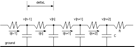
Finite-element difference equations (without midpoint rule correction):
   tnow += deltaT;
   for (n in ...) i[n] = (v[n-1]-v[n])/R;
   for (n in ...) v[n] += (i[n]-i[n+1])*deltaT/C;

Basic finite-difference simulation uses fixed spatial grid (element size is deltaL) and fixed time step (deltaT seconds).

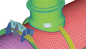
Each grid point holds a vector of instantatious local properties, such as voltage, temperature, stress, pressure, magnetic flux.

Physical quantities are divided over the grid. Three examples:

Sound wave in wire: C=deltaL*mass-per-unit-length, R=deltaL*elasticity-per-unit-length
Heat wave in wire: C=deltaL*heat-capacity-per-unit-length, R=deltaL*thermal-conductance-per-unit-length
Electrical wave in wire: C=deltaL*capacitance-per-unit-length, R=deltaL*resistance-per-unit-length

Larger modelling errors with larger deltaT and deltaL, but faster simulation. Keep them less than 1/10th wavelength for good accuracy. Generally use a 2D or 3D grid for fluid modelling: 1D ok for electronics.

Typically want to model both resistance and inductance for electrical system.

When modelling inductance instead of resistance, then need a `+=' in the i[n] equation.

When non-linear components are present (e.g. diodes and FETs), SPICE simulator adjusts deltaT dynamically depending on point in the curve. Finite element simulation is not examinable for Part II System-on-Chip.