Luminance of a square

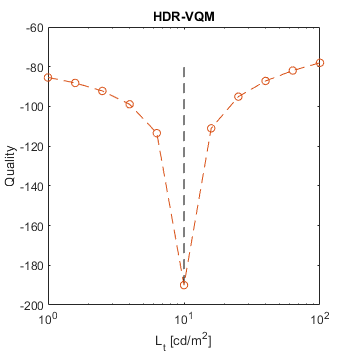
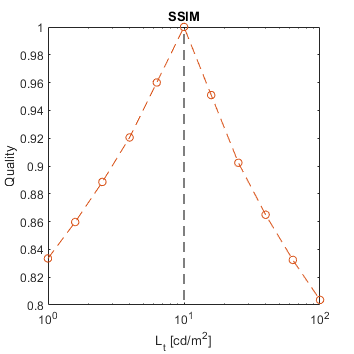
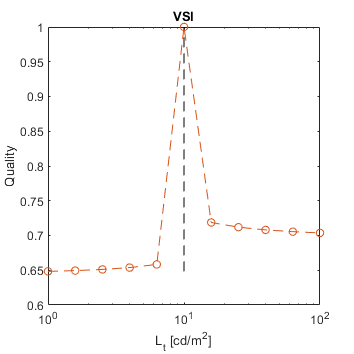
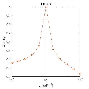
A square of varying luminance level (from 1 to 100 cd/m²) was added to a uniform background of 10cd/m². This example shows how metrics scale large luminance contrast.

Note the asymmetry between darker (left side of the plot) and brighter square that is modelled by some of the metrics. The further level of darkness tend to be less discriminable.

See the test image gallery.

test_band_lim_noise

See the test image gallery.

Blur

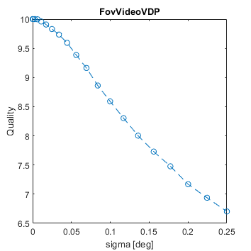
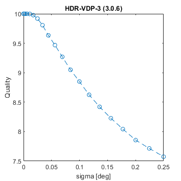
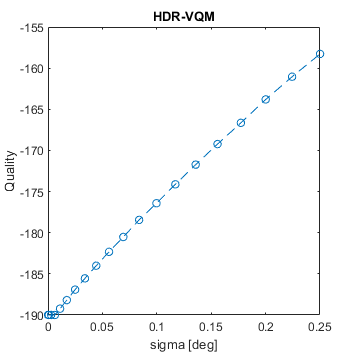
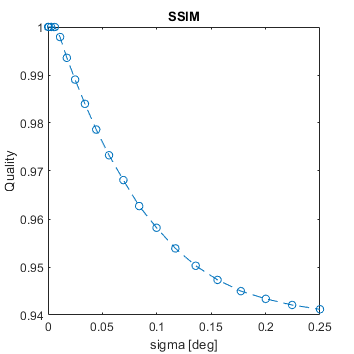
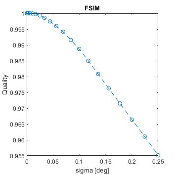
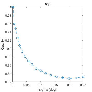
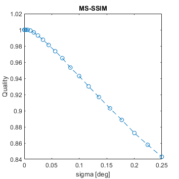
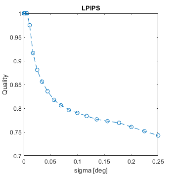
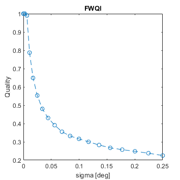
An image with a square was blurred using a Gaussian filter with a given sigma (in terms of visual degrees). The assumed resolution was 50 ppd.

See the test image gallery.

Noise

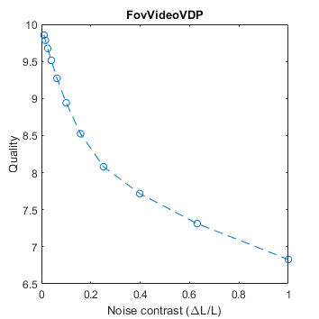
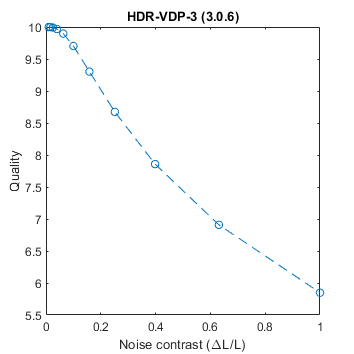
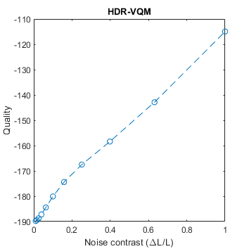
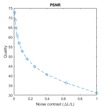
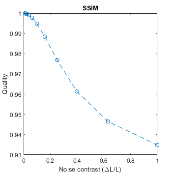
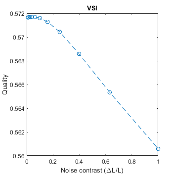
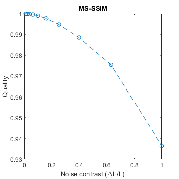
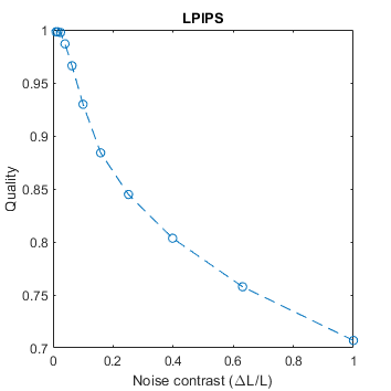
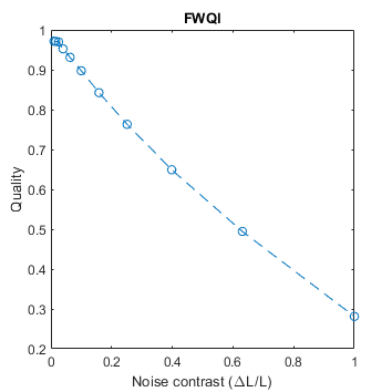
A square with an increasing amplitude of white uniformly distributed noise was added to an images. The noise amplitude is reported in the units of Michelson contrast.

See the test image gallery.

Size of a noise pattern

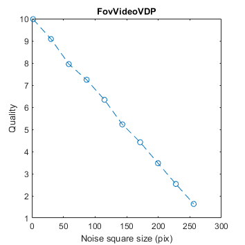
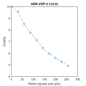
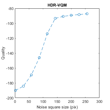
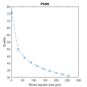
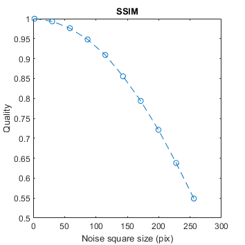
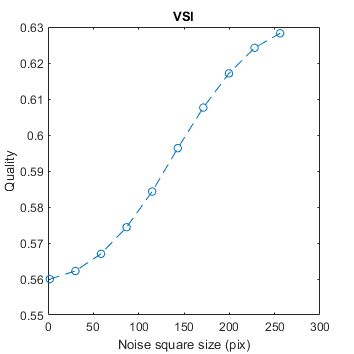
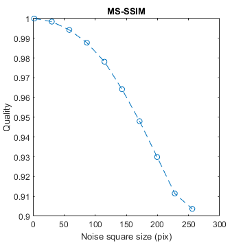
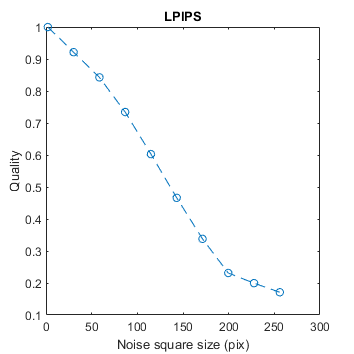
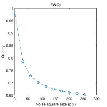
A square with white uniformly distributed noise is increasing in size. Large distortions tend to be more objectionable. The noise has the contrast of 0.3. The size is reported as with with/height of an edge.

This example tests how metrics scale the quality with the size of a distortion.

See the test image gallery.

JPEG compression distortions

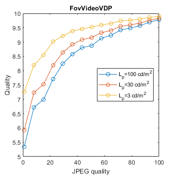
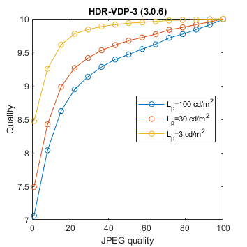
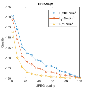
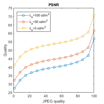
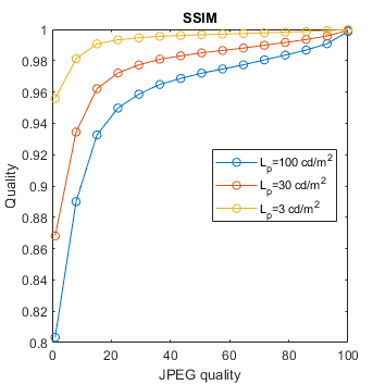
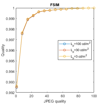
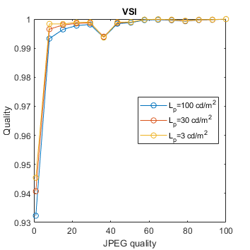
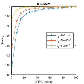
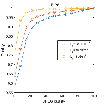
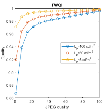
An image is compressed at different quality setting of JPEG. Additionally, is displayed at three display brightness levels. Distortions tend to be less noticeable on darker displays, but not every metric can account for that.

See the test image gallery.

JPEG encoded image seen from different viewing distances

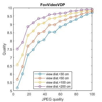
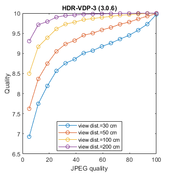
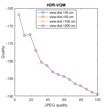
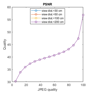
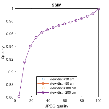
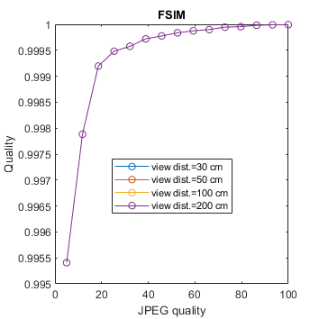
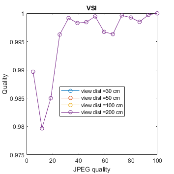
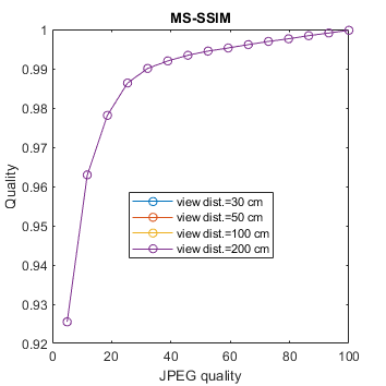
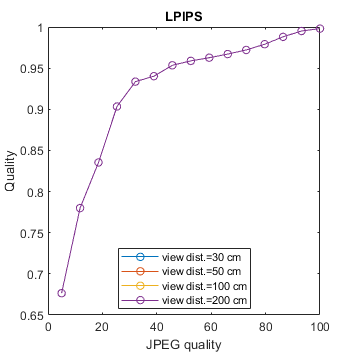
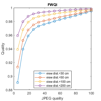
An image is encoded with JPEG and seen from different viewing distances. Only the metrics that account for the physical size of the display can predict that distortions are less visible (have lesser impact on quality) when seen from larger viewing distances.

See the test image gallery.

Estimating quality degradation due to standard distortions

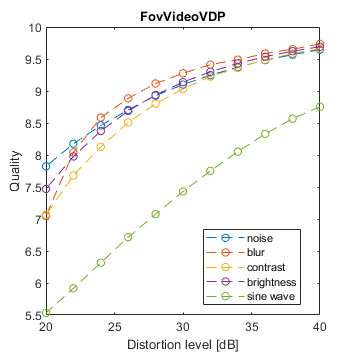
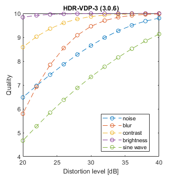
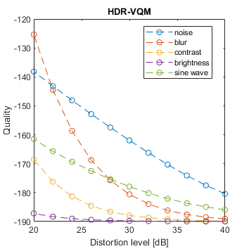
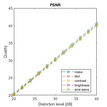
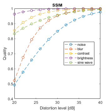
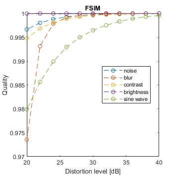
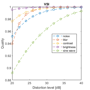
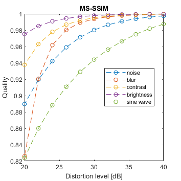
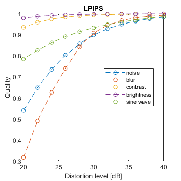
One of five typical distortions was introduced to an image: noise, blur, contrast change, brightness change and a sinusoidal pattern. The levels of the distortions were selected so that the distorted images resulted in a fixed PSNR value. The images that are reported to have the same distortion level in terms of PSNR, may have very different perceived level of distortion. For example, the change of brightness causes the large change of PSNR, but almost unnoticeable change in an image. This is an example of failure of PSNR and also some other metrics.

Note that the distortion due to sine wave is the most noticeable and that noisy images look better than blurry images at the same PSNR value.

See the test image gallery.

Contrast sensitivity function for Gabor patches

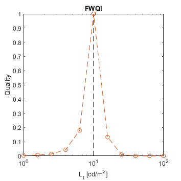
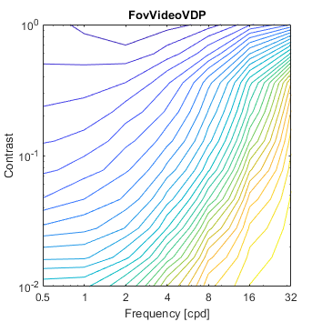
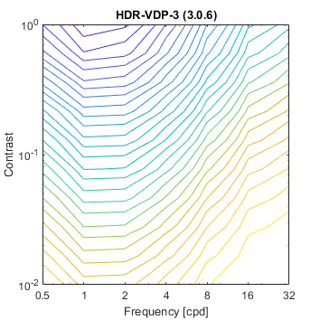
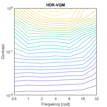
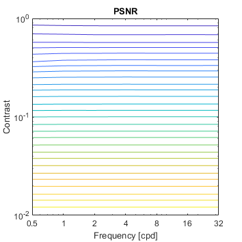
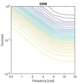
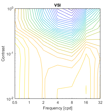
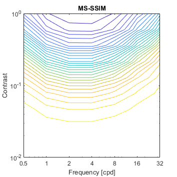
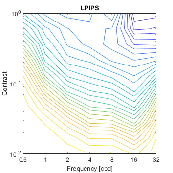
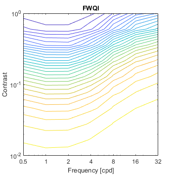
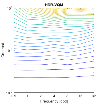
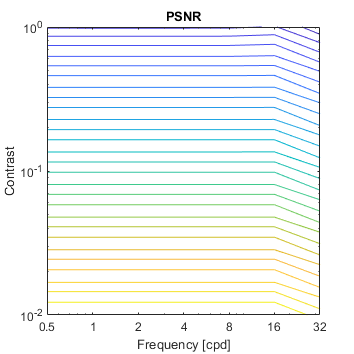
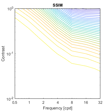
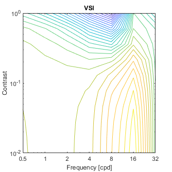
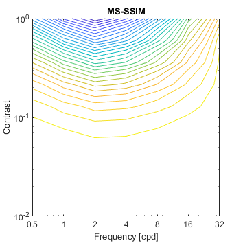
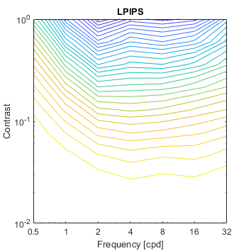
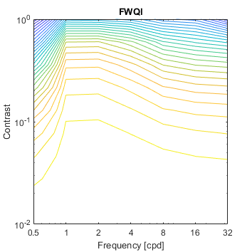
This example consists of a matrix of Gabor patches of varying frequency and contrast. It tests metrics ability to predict contrast sensitivity function.

Note that simple metrics, such as PSNR respond the same regardless of the frequency. SSIM is the most sensitive to the highest frequencies but MS-SSIM is addressing this issue by shifting the peak sensitivity to about 2-3 cpd. Some metrics (VSI, FWQI) have a rather arbitrary response to such Gabor patterns.

See the test image gallery.

Contrast masking

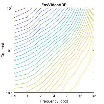
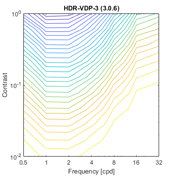
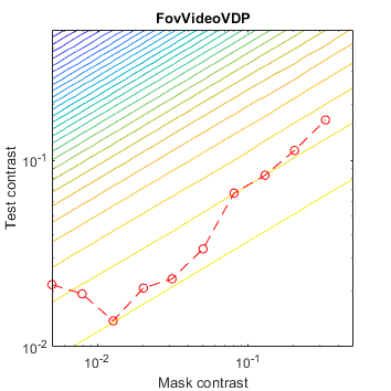
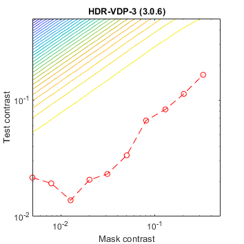
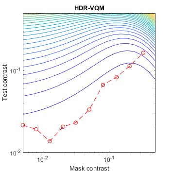
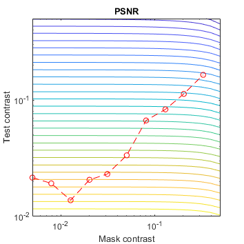
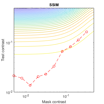
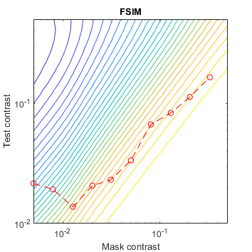
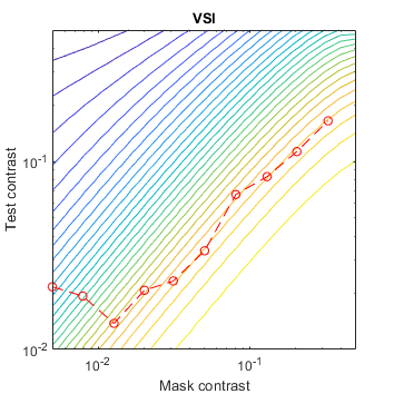
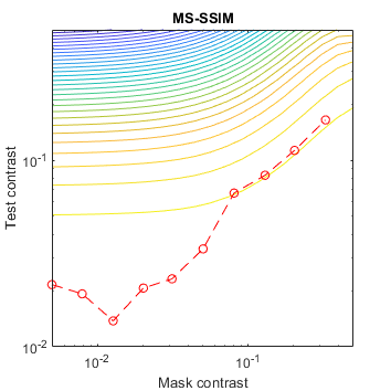
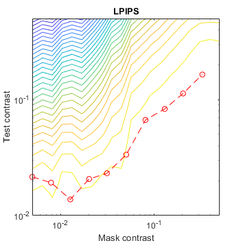
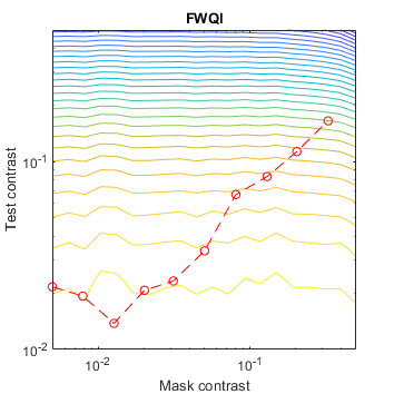
The test stimuli consists of a matrix of Gabor patches superimposed on a sinusoidal grating. The grating acts as a masker for the Gabour patch, making it less visible when the contrast of the grating is high. This is a traditional stimuli for measuring the effect of contrast masking.

The contour lines shows the response of a metric for a given contrast of a masker and the test Gabor patch. The red line represent measured discrimination thresholds from the paper "Human luminance pattern-vision mechanisms: masking experiments require a new model," J. Opt. Soc. Am. A 11, 1710-1719 (1994) DOI

Metrics that do not explicitly model contrast masking often indirectly account for masking, as this is one of the fundamental phenomena that dictates the visibility of artifacts. However, some metrics show more irregularities than the others.

See the test image gallery.

Localized flicker

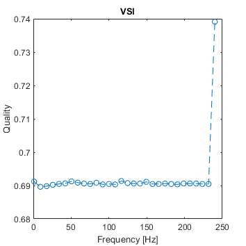
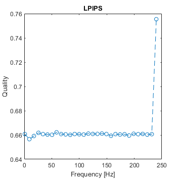
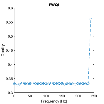
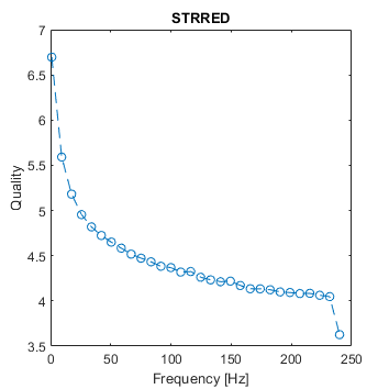
A flickering artifacts was introduced in one corner of the image. The frequency of the flicker was varied.

Most metrics cannot account for the frequency of the flicker.

Flicker

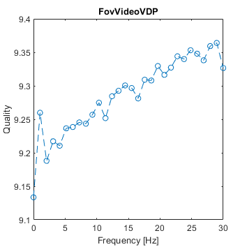
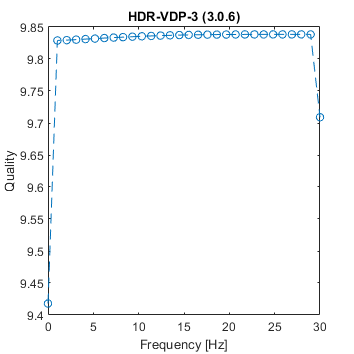
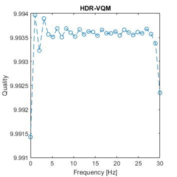
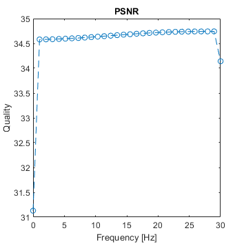
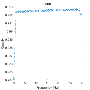
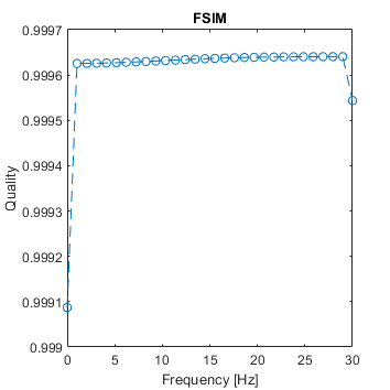
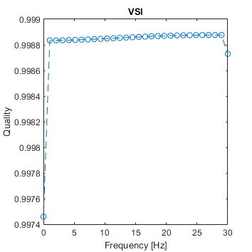
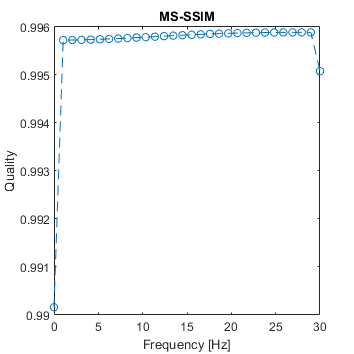
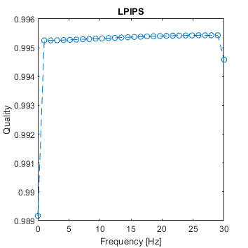
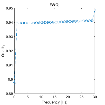
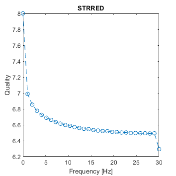
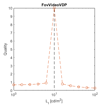
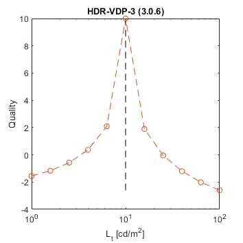
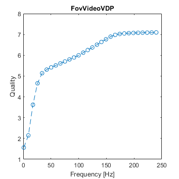
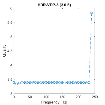
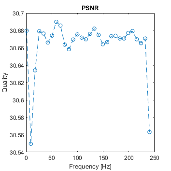
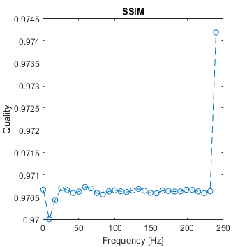
A square changes its brightness over time with a given frequency. The brightness is modulated using a cosine function. The contrast of the modulation is 0.5. The reference video is a uniform field of 10 cd/m².

Only FovVideoVDP can predict the distortion due to flicker and also the frequency at which the flicker is fused.

Eccentricity

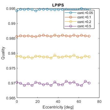
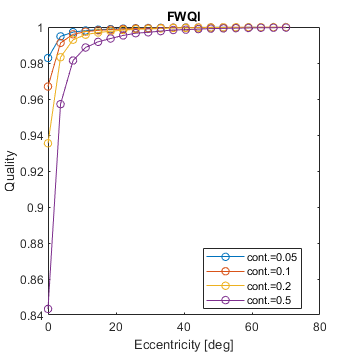
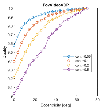
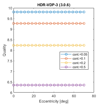
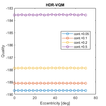
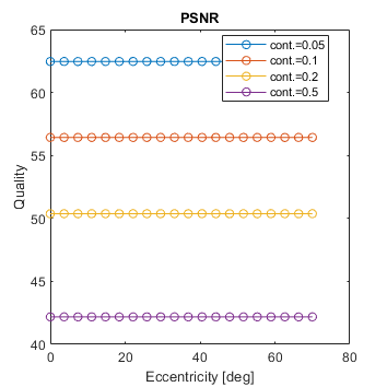
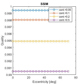
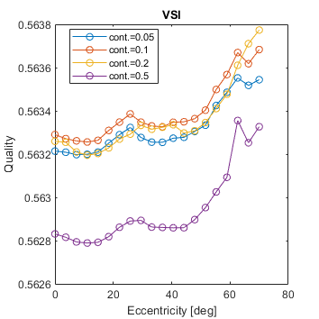
A noisy square is shown at different eccentricities. The noise of different contrast is generated.

Not surprisingly, only the metrics that account for foveated viewing can predict the effect of eccentricity.

See the test image gallery.