Preface
Summary
Natural numbers, Peano’s axioms and Peano structures
Algebras and coalgebras
Coinduction and bisimulation
- Bisimulation coinduction for conumbers
  - Example of bisimulation coinduction for numbers
  - Justification of bisimulation coinduction for numbers
- Bisimulation coinduction for lists
  - Examples of bisimulation coinduction for lists
  - Justification of bisimulation coinduction for lists
${{\Bbb{F}}}$-algebras and ${{\Bbb{F}}}$-coalgebras
Least and greatest fixed points
Use in programming
Concluding thoughts

$\phantom{}$
$\phantom{}$
This article is meant to be read in a browser, but the web page can take several minutes to load because MathJax is slow. The PDF version is quicker to load, but the latex generated by Pandoc is not as beautifully formatted as it would be if it were from bespoke ${\small{\LaTeX}}$.

Preface

For a long time I’ve been aware of corecursion and coinduction as something mysteriously dual to recursion and induction, and related to maximal fixed points and bisimulation … but I’ve never understood what they are or what the duality signified by the “co” means. My goal here is to try to understand these things through the activity of creating a simple explanation.

Early drafts of this article were rather formal and included proofs of everything – I even started to check some of the details with a proof assistant to try to increase my confidence that I’d got them right. After a while I realised that the writing was taking too long. Furthermore, the notational infrastructure needed for fully rigorous formal precision was obscuring the essence of the ideas. I also realised that the thing I was producing was in danger of ending up as an amateur and inferior version of existing expositions, so I decided to scale back on mathematical precision and largely give up on including formal proofs. A result of this is that I make assertions that I haven’t checked in detail, so there are bound to be errors, technical mistakes and embarrassing omissions and misunderstandings. If you happen to be reading this and spot any of these, then please let me know!

To get started, I did some googling and found the link What the heck is coinduction and a couple of excellent tutorials:

A Tutorial on Co-induction and Functional Programming by Andy Gordon.
An introduction to (co)algebra and (co)induction by Bart Jacobs and Jan Rutten;

I also spotted a new book Introduction to Coalgebra by Bart Jacobs whilst browsing in the Cambridge CUP bookshop – subsequent googling discovered a preliminary version of this online here.

It’s a small world: in the distant past both Andy Gordon and Bart Jacobs worked as postdocs on grants for which I was one of the investigators. I think this was long before either of them became authorities on coinduction.

There is nothing new here. The material is adapted from several sources, particularly those mentioned above, as well as other papers and web pages that I stumbled across and found enlightening – links to some of these are included in the text. I mostly didn’t read these beyond the introductory and motivational parts, so it’s inevitable that I’ve misunderstood some things. As my sources are just those I happened to find, there might be better ones I could have read and cited. Please let me know if you have any suggestions.

Summary

The first three sub-sections of this summary are an example-based preview illustrating some of the core ideas covered in the rest of the article as they apply to lists. In particular:

lists and their constructors versus
colists and their destructors;
recursion on finite lists versus
corecursion on finite or infinite colists;
the relation of least fixed points to lists and induction versus
the relation of greatest fixed points to colists and bisimulation coinduction.

The summary concludes with a fourth sub-section that itemises the topics covered in the remainder of the article.

Recursion and induction are most familiar for natural numbers, but corecusion and coinduction for numbers are pretty useless and I couldn’t find illustrative examples that didn’t seem vacuous – this is why I focus on lists in this summary. However, the main part of this article is about concepts rather than examples and it starts with numbers, as they provide a minimal setting for explaining some of the core ideas. Lists can then be seen as a generalisation, as well a providing examples that hint at useful applications. Lists are also a nice stepping stone to a superficial account of the general frameworks of algebras and coalgebras and then ${{\Bbb{F}}}$-algebras and ${{\Bbb{F}}}$-coalgebras.

The material in the sections following the summary provides more explanation and details, starting with corecursion and coinduction for numbers. At the end there are brief and superficial discussions of how the number and list examples fit into the more general framework of algebras and coalgebras, and then how this relates to programming language datatypes and function definitions on these types.

Data, codata, constructors and destructors

Data represents finite values and is built by evaluating a finite number of applications of constructor functions. Codata often – but not necessarily – represents infinite values and is defined by specifying the values of destructor functions. Here are two examples.

Data: The 4-element finite list ${\small\mathsf{L}}_4={\mathbf{\small{[}}}1,1,1,1{\mathbf{\small{]}}}$ is built by specifying
${\small\mathsf{L}}_4={{\mathsf{cons}}}(1,{{\mathsf{cons}}}(1,{{\mathsf{cons}}}(1,{{\mathsf{cons}}}(1,{{\mathsf{nil}}}))))$, where ${{\mathsf{cons}}}$ is a list constructor and ${{\mathsf{nil}}}$, the empty list, a nullary constructor.
Codata: The infinite list ${\small\mathsf{L}}_{\tiny\infty}={\mathbf{\small{[}}}1,1,1,1,\ldots{\mathbf{\small{]}}}$ is defined by specifying
${{\mathsf{hd}}}({\small\mathsf{L}}_{\tiny\infty}){\,{=}\,}{1}$ and ${{\mathsf{tl}}}({\small\mathsf{L}}_{\tiny\infty}){\,{=}\,}{{\small\mathsf{L}}_{\tiny\infty}}$, where ${{\mathsf{hd}}}$ and ${{\mathsf{tl}}}$ are destructors.

Recursion and corecursion

Recursion defines a function mapping values from a datatype by invoking itself on the components of the constructors used to build data values. Corecursion defines a function mapping to a codatatype by specifying the results of applying destructors to the results of the function. This is illustrated with examples using finite and infinite lists.

Let ${{\Bbb N}}$ be the set of natural numbers, ${{\Bbb L}}$ be the set of finite lists of numbers and ${{{\Bbb L}}_{\infty}}$ the set of infinite lists of numbers. Let ${{\overline{{{\Bbb L}}}}}={{\Bbb L}}\cup{{{\Bbb L}}_{\infty}}$ be the set of finite or infinite lists of numbers.

The list constructors are ${{\mathsf{nil}}}$ and ${{\mathsf{cons}}}$: ${{\mathsf{nil}}}$ is the empty list and ${{\mathsf{cons}}}(n,l)$ is the list constructed by adding the number $n$ to the front of list $l$.

The list destructors are ${{\mathsf{null}}}$, ${{\mathsf{hd}}}$ and ${{\mathsf{tl}}}$: ${{\mathsf{null}}}(l)$ is true if and only $l{\,{=}\,}{{\mathsf{nil}}}$, ${{\mathsf{hd}}}(l)$ is the first element of $l$ and ${{\mathsf{tl}}}(l)$ is the list resulting from removing its first element. The equation $l={{{\mathtt{if}}}~{{\mathsf{null}}}(l)~{{\mathtt{then}}}~{{\mathsf{nil}}}~{{\mathtt{else}}}~{{\mathsf{cons}}}({{\mathsf{hd}}}(l),{{\mathsf{tl}}}(l))}$ holds for every list $l$.

In what follows, the functions ${\pi_1}:X_1{\times}X_2{{\;{\to}\;}}X_1$ and ${\pi_2}:X_1{\times}X_2{{\;{\to}\;}}X_2$ extract the first and second elements of pairs: ${\pi_1}(x_1,x_2){\,{=}\,}x_1$ and ${\pi_2}(x_1,x_2){\,{=}\,}x_2$. The notation $A\Leftrightarrow B$ means $A$ is true if and only if $B$ is true.

Example. The function ${{\small\mathsf{Add1}}}$ adds $1$ to each element of a list of numbers and is defined below both by recursion and corecursion. The recursively defined ${{\small\mathsf{Add1}}}$ maps finite lists to finite lists, so ${{\small\mathsf{Add1}}}:{{\Bbb L}}{{\;{\to}\;}}{{\Bbb L}}$. The corecursively defined ${{\small\mathsf{Add1}}}$ maps finite lists to finite lists and infinite lists to infinite lists, so ${{\small\mathsf{Add1}}}:{{\overline{{{\Bbb L}}}}}{{\;{\to}\;}}{{\overline{{{\Bbb L}}}}}$.

Recursion:
${{\small\mathsf{Add1}}}({{\mathsf{nil}}})={{\mathsf{nil}}}$ and ${{\small\mathsf{Add1}}}({{\mathsf{cons}}}(n,l))={{\mathsf{cons}}}(n{+}1,{{\small\mathsf{Add1}}}(l))$
Corecursion:
${{\mathsf{null}}}({{\small\mathsf{Add1}}}(l))\,{=}\,(l{=}{{\mathsf{nil}}})\,$and$\,{{\mathsf{hd}}}({{\small\mathsf{Add1}}}(l))\,{=}\,{{\mathsf{hd}}}(l){+}1\,$and$\,{{\mathsf{tl}}}({{\small\mathsf{Add1}}}(l))\,{=}\,{{\small\mathsf{Add1}}}({{\mathsf{tl}}}(l))$

More generally, recursion defines functions from ${{\Bbb L}}$ to some set $X$, whereas corecursion defines functions from some set $X$ to ${{\overline{{{\Bbb L}}}}}$.

If $x_0\in X$ and $\theta:{{\Bbb N}}{\times}X{{\;{\to}\;}}X$, then $f:{{\Bbb L}}{{\;{\to}\;}}X$ is defined by recursion by:
$~~~f(l)={{{\mathtt{if}}}~l{\,{=}\,}{{\mathsf{nil}}}~{{\mathtt{then}}}~x_0~{{\mathtt{else}}}~\theta({{\mathsf{hd}}}(l),f({{\mathsf{tl}}}(l))}$
which specifies the result of applying $f$ to values build using constructors:
$~~~f({{\mathsf{nil}}}){\,{=}\,}x_0$ and $f({{\mathsf{cons}}}(n,l)){\,{=}\,}\theta(n,f(l))$

If ${\small{P}}\subseteq X$ and $\phi:X{{\;{\to}\;}}{{\Bbb N}}{\times}X$, then $g:X{{\;{\to}\;}}{{\overline{{{\Bbb L}}}}}$ is defined by corecursion by:
$~~~g(x)={{{\mathtt{if}}}~x\,{\in}{\small{P}}~{{\mathtt{then}}}~{{\mathsf{nil}}}~{{\mathtt{else}}}~{{\mathsf{cons}}}({\pi_1}(\phi(x)), g({\pi_2}(\phi(x))))}$
which determines the result of applying the destructors to $g(x)$:
$~~~{{\mathsf{null}}}(g(x))\Leftrightarrow x\,{\in}\,{\small{P}}$ and ${{\mathsf{hd}}}(g(x)){\,{=}\,}{\pi_1}(\phi(x))$ and ${{\mathsf{tl}}}(g(x)){\,{=}\,}g({\pi_2}(\phi(x)))$

Returning to the ${{\small\mathsf{Add1}}}$ example, recall the equation:

$~~~{{\small\mathsf{Add1}}}(l) = {{{\mathtt{if}}}~l{\,{=}\,}{{\mathsf{nil}}}~{{\mathtt{then}}}~{{\mathsf{nil}}}~{{\mathtt{else}}}~{{\mathsf{cons}}}({{\mathsf{hd}}}(l){+}1,{{\small\mathsf{Add1}}}({{\mathsf{tl}}}(l)))}$

This can be viewed as a definition by recursion by taking $f{\,{=}\,}{{\small\mathsf{Add1}}}$, $X{\,{=}\,}{{\Bbb L}}$, $x_0{\,{=}\,}{{\mathsf{nil}}}$ and $\theta(n,l){\,{=}\,}{{\mathsf{cons}}}(n{+}1,l)$ in the recursion scheme for $f$ in the first bullet point above.

It can be viewed as a definition by corecursion by taking $g{\,{=}\,}{{\small\mathsf{Add1}}}$, $X{\,{=}\,}{{\overline{{{\Bbb L}}}}}$, ${\small{P}}{\,{=}\,}\{{{\mathsf{nil}}}\}$ and $\phi(l){\,{=}\,}({{\mathsf{hd}}}(l){+}1,{{\mathsf{tl}}}(l))$ in corecursion scheme for $g$ in the second bullet point.

The version of ${{\small\mathsf{Add1}}}$ defined by recursion maps ${{\Bbb L}}$ to ${{\Bbb L}}$, so only finite lists can be arguments and results, but the version defined by corecursion maps ${{\overline{{{\Bbb L}}}}}$ to ${{\overline{{{\Bbb L}}}}}$, which allows both finite and infinite lists to be arguments and results.

This sub-section concludes with three examples of corecursion that will reappear later.

Example. The function ${{\small\mathsf{CountFrom}}}:{{\Bbb N}}{{\;{\to}\;}}{{\overline{{{\Bbb L}}}}}$ maps a number to an infinite list, i.e. to a member of the ${{{\Bbb L}}_{\infty}}$ subset of ${{\overline{{{\Bbb L}}}}}$.

$~~~{{\small\mathsf{CountFrom}}}(n)~=~{{\mathsf{cons}}}(n,{{\small\mathsf{CountFrom}}}(n{+}1))$

This corecursion equation defines ${{\small\mathsf{CountFrom}}}(n)$ to be the infinite list counting up from $n$, i.e. ${{\mathsf{cons}}}(n,{{\mathsf{cons}}}(n{+}1,{{\mathsf{cons}}}(n{+}2,\ldots)))$. If $X{\,{=}\,}{{\Bbb N}}$, ${\small{P}}$ is the empty set and $\phi(n){\,{=}\,}(n,n{+}1)$, then ${{\small\mathsf{CountFrom}}}{\,{=}\,}{g}$, where $g$ is defined by corecursion by the single corecursion equation:

$~~~g(x)={{{\mathtt{if}}}~x\,{\in}{\small{P}}~{{\mathtt{then}}}~{{\mathsf{nil}}}~{{\mathtt{else}}}~{{\mathsf{cons}}}({\pi_1}(\phi(x)), g({\pi_2}(\phi(x))))}$

${{\small\mathsf{CountFrom}}}$ can also be specified by giving equations for the destructors:

$~~~\begin{array}{ll} {{\mathsf{null}}}({{\small\mathsf{CountFrom}}}(n)) &\!\!\!\!\!= ~\text{false} \\ {{\mathsf{hd}}}({{\small\mathsf{CountFrom}}}(n)) &\!\!\!\!\!= ~n \\ {{\mathsf{tl}}}({{\small\mathsf{CountFrom}}}(n)) &\!\!\!\!\!= ~{{\small\mathsf{CountFrom}}}(n{+}1) \end{array}$

Example. The function ${{\small\mathsf{CountUp}}}:{{\Bbb N}}{\times}{{\Bbb N}}{{\;{\to}\;}}{{\overline{{{\Bbb L}}}}}$ maps a pair of numbers $(m,n)$ to a finite list when $m\leq n$ and to an infinite lists when $m > n$.

$~~~{{\small\mathsf{CountUp}}}(m,n)~=~{{{\mathtt{if}}}~m{\,{=}\,}{n}~{{\mathtt{then}}}~{{\mathsf{nil}}}~{{\mathtt{else}}}~{{\mathsf{cons}}}(m,{{\small\mathsf{CountUp}}}(m{+}1,n))}$

If $m\leq n$, then this corecursion equation defines ${{\small\mathsf{CountUp}}}(m,n)$ to be the finite list counting up from $m$ until $n$ (including $m$ but not $n$, so ${{\small\mathsf{CountUp}}}(m,m){\,{=}\,}{{\mathsf{nil}}}$ and ${{\small\mathsf{CountUp}}}(m,m{+}1){\,{=}\,}{{\mathsf{cons}}}(m,{{\mathsf{nil}}})$).

If $m > n$, then the equation defines ${{\small\mathsf{CountUp}}}(m,n)$ to be the infinite list counting up from $m$.

If $X{\,{=}\,}{{\Bbb N}}{\times}{{\Bbb N}}$, ${\small{P}}{\,{=}\,}\{(m,n)\mid m{\,{=}\,}n\}$ and $\phi(m,n){\,{=}\,}(m,(m{+}1,n))$, then ${{\small\mathsf{CountUp}}}{\,{=}\,}{g}\textsf{,}$ where $g$ is defined by corecursion by the single corecursion equation:

$~~~g(x) = {{{\mathtt{if}}}~x\,{\in}{\small{P}}~{{\mathtt{then}}}~{{\mathsf{nil}}}~{{\mathtt{else}}}~{{\mathsf{cons}}}({\pi_1}(\phi(x)),g({\pi_2}(\phi(x))))}$

${{\small\mathsf{CountUp}}}$ can also be specified by giving equations for the destructors:

$~~~\begin{array}{ll} {{\mathsf{null}}}({{\small\mathsf{CountUp}}}(m,n)) &\!\!\!\!\!= ~(m{\,{=}\,}n) \\ {{\mathsf{hd}}}({{\small\mathsf{CountUp}}}(m,n)) &\!\!\!\!\!= ~m \phantom{{{\small\mathsf{CountUp}}}({+}1,n)}~~~~\text{if}~~m\neq n\\ {{\mathsf{tl}}}({{\small\mathsf{CountUp}}}(m,n)) &\!\!\!\!\!= ~{{\small\mathsf{CountUp}}}(m{+}1,n) ~~~~\text{if}~~m\neq n \\ \end{array}$

Example. The function ${{\small\mathsf{CountUpTo}}}:{{\Bbb N}}{\times}{{\Bbb N}}{{\;{\to}\;}}{{\overline{{{\Bbb L}}}}}$ maps a pair of numbers to a finite lists, i.e. to a member of the ${{\Bbb L}}$ subset of ${{\overline{{{\Bbb L}}}}}$.

$~~~{{\small\mathsf{CountUpTo}}}(m,n)~=~{{{\mathtt{if}}}~m\geq{n}~{{\mathtt{then}}}~{{\mathsf{nil}}}~{{\mathtt{else}}}~{{\mathsf{cons}}}(m,{{\small\mathsf{CountUpTo}}}(m{+}1,n))}$

If $m\leq n$ then this corecursion equation defines ${{\small\mathsf{CountUp}}}(m,n)$ to be the finite list counting up from $m$ until $n$ (including $m$ but not $n$. If $m>n$, then ${{\small\mathsf{CountUp}}}(m,n){\,{=}\,}{{\mathsf{nil}}}$.

If $X{\,{=}\,}{{\Bbb N}}{\times}{{\Bbb N}}$, ${\small{P}}{\,{=}\,}\{(m,n)\mid m\geq n\}$ and $\phi(m,n){\,{=}\,}(m,(m{+}1,n))$, then ${{\small\mathsf{CountUpTo}}}{\,{=}\,}{g}$, where $g$ is defined by corecursion by the single corecursion equation:

$~~~g(x) = {{{\mathtt{if}}}~x\,{\in}{\small{P}}~{{\mathtt{then}}}~{{\mathsf{nil}}}~{{\mathtt{else}}}~{{\mathsf{cons}}}({\pi_1}(\phi(x)),g({\pi_2}(\phi(x))))}$

${{\small\mathsf{CountUpTo}}}$ can also be specified by giving equations for the destructors:

$~~~\begin{array}{ll} {{\mathsf{null}}}({{\small\mathsf{CountUpTo}}}(m,n)) &\!\!\!\!\!= ~(m\geq n) \\ {{\mathsf{hd}}}({{\small\mathsf{CountUpTo}}}(m,n)) &\!\!\!\!\!= ~m \phantom{{{\small\mathsf{CountUpTo}}}({+}1,n)}~~~~\text{if}~~m < n\\ {{\mathsf{tl}}}({{\small\mathsf{CountUpTo}}}(m,n)) &\!\!\!\!\!= ~{{\small\mathsf{CountUpTo}}}(m{+}1,n) ~~~~\text{if}~~m < n \end{array}$

Fixed points, induction, coinduction and bisimulation

A fixed point of a function $\theta$ is an $x$ such that $\theta(x){\,{=}\,}x$.

If $L \subseteq {{\overline{{{\Bbb L}}}}}$, define ${\cal F}(L) = \{{{\mathsf{nil}}}\}\cup\{{{\mathsf{cons}}}(n,l)\mid n\in{{\Bbb N}}~\text{and}~ l\in L\}$.

${{\Bbb L}}$ and ${{\overline{{{\Bbb L}}}}}$ are both fixed points of ${\cal F}$, i.e. ${\cal F}({{\Bbb L}}){\,{=}\,}{{\Bbb L}}$ and ${\cal F}({{\overline{{{\Bbb L}}}}}){\,{=}\,}{{\overline{{{\Bbb L}}}}}$. The least fixed point is ${{\Bbb L}}$ and the greatest fixed point is ${{\overline{{{\Bbb L}}}}}$.

${{\Bbb L}}$ is also the least pre-fixed point of ${\cal F}$, that is the least $L\subseteq {{\overline{{{\Bbb L}}}}}$ such that ${\cal F}(L) \subseteq L$. Thus if ${\cal F}(L) \subseteq L$ then by leastness ${{\Bbb L}}\subseteq L$. This is the principle of induction for finite lists since ${\cal F}(L) \subseteq L$ is equivalent to ${{\mathsf{nil}}}\in L$ (the base case of the induction) and $\forall n\in{{\Bbb N}}.\,\forall l\in L.\,{{\mathsf{cons}}}(n,l)\in L$ (the induction step). ${{\Bbb L}}\subseteq L$ is equivalent to $\forall l\in{{\Bbb L}}.\,l\in L$.

${{\overline{{{\Bbb L}}}}}$ is also the greatest post-fixed point of ${\cal F}$, that is the greatest $L\subseteq {{\overline{{{\Bbb L}}}}}$ such that $L\subseteq {\cal F}(L)$, but there doesn’t seem to be any interesting reasoning principle arising from this. The principle dual to induction is: if $L\subseteq {\cal F}(L)$ then by greatestness $L\subseteq{{\overline{{{\Bbb L}}}}}$ – but this is vacuous as $L\subseteq{{\overline{{{\Bbb L}}}}}$ is assumed.

However, there is a useful reasoning principle for binary relations on ${{\overline{{{\Bbb L}}}}}$ that is derived from greatest fixed points. This is the main coinduction principle and is based on subsets of ${{\overline{{{\Bbb L}}}}}{\times}{{\overline{{{\Bbb L}}}}}$ rather than subsets of just ${{\overline{{{\Bbb L}}}}}$.

If $R\subseteq {{\overline{{{\Bbb L}}}}}{\times}{{\overline{{{\Bbb L}}}}}$ is a binary relation on ${{\overline{{{\Bbb L}}}}}$, then define ${{{\cal B}}}(R)\subseteq {{\overline{{{\Bbb L}}}}}{\times}{{\overline{{{\Bbb L}}}}}$ by:

${{{\cal B}}}(R) = \{({{\mathsf{nil}}},{{\mathsf{nil}}})\} \cup \{({{\mathsf{cons}}}(n,l_1),{{\mathsf{cons}}}(n,l_2))\mid n\in{{\Bbb N}}\wedge (l_1,l_2)\in R\}$

The least fixed point of ${{{\cal B}}}$ is the equality relation on ${{\Bbb L}}$, i.e. $\{(l,l)\mid l\in{{\Bbb L}}\}$, and the greatest fixed point is the equality relation on ${{\overline{{{\Bbb L}}}}}$, i.e. $\{(l,l)\mid l\in{{\overline{{{\Bbb L}}}}}\}$.

The relation $\{(l,l)\mid l\in{{\overline{{{\Bbb L}}}}}\}$ is also the greatest post-fixed point of ${{{\cal B}}}$, that is the greatest $R$ such that $R\subseteq {{\cal B}}(R)$. Thus if there exists an $R$ such that $R\subseteq {{\cal B}}(R)$, then by greatestness $R\subseteq\{(l,l)\mid l\in{{\overline{{{\Bbb L}}}}}\}$. This is a principle of coinduction.

The property $R\subseteq {{{\cal B}}}(R)$ means that if $(l_1,l_2)\in R$ then either $l_1{\,{=}\,}{{\mathsf{nil}}}$ and $l_2{\,{=}\,}{{\mathsf{nil}}}$ or else $l_1{\,{=}\,}{{\mathsf{cons}}}(n,l_1')$ and $l_2{\,{=}\,}{{\mathsf{cons}}}(n,l_2')$ and $(l'_1,l_2')\in R$, for some $n\in{{\Bbb N}}$ and $l_1',l_2'\in{{\overline{{{\Bbb L}}}}}$. Such an $R$ is called a bisimulation.

The proof principle that if $R$ is a bisimulation then $\forall l_1\,l_2\in{{\overline{{{\Bbb L}}}}}.\,(l_1,l_2)\in R {\;\Rightarrow\;}l_1{\,{=}\,}l_2$ is called bisumulation coinduction here, or just coinduction, which is the more common name for this principle.

Recall the corecursively defined functions:

$\begin{array}{ll} {{\small\mathsf{CountFrom}}}(n) &\!\!\!\!\!=~{{\mathsf{cons}}}(n,{{\small\mathsf{CountFrom}}}(n{+}1))\\ {{\small\mathsf{CountUp}}}(m,n) &\!\!\!\!\!=~{{{\mathtt{if}}}~m=n~{{\mathtt{then}}}~{{\mathsf{nil}}}~{{\mathtt{else}}}~{{\mathsf{cons}}}(m,{{\small\mathsf{CountUp}}}(m{+}1,n))}\\ {{\small\mathsf{CountUpTo}}}(m,n) &\!\!\!\!\!=~{{{\mathtt{if}}}~m\geq{n}~{{\mathtt{then}}}~{{\mathsf{nil}}}~{{\mathtt{else}}}~{{\mathsf{cons}}}(m,{{\small\mathsf{CountUpTo}}}(m{+}1,n))} \end{array}$

Examples of bisimulations are $R_1$ and $R_2$, where:

$\begin{array}{lll} R_1 &\!\!=~ \{({{\small\mathsf{CountUp}}}(m,n),{{\small\mathsf{CountFrom}}}(m)) &\!\!\!\!\!\mid~ m>n\}\\ R_2 &\!\!=~ \{({{\small\mathsf{CountUp}}}(m,n),{{\small\mathsf{CountUpTo}}}(m,n))&\!\!\!\!\!\mid~ m\leq n\} \end{array}$

The easy arguments that $R_1$ and $R_2$ are bisimulations are given at the beginning of the section on examples of bisimulation coinduction for lists.

By bisimulation coinduction applied to $R_1$:
$\forall m\,n\in{{\Bbb N}}.\, m>n {\;\Rightarrow\;}{{\small\mathsf{CountUp}}}(m,n){\,{=}\,}{{\small\mathsf{CountFrom}}}(m)$.

By bisimulation coinduction applied to $R_2$:
$\forall m\,n\in{{\Bbb N}}.\, m\leq n {\;\Rightarrow\;}{{\small\mathsf{CountUp}}}(m,n){\,{=}\,}{{\small\mathsf{CountUpTo}}}(m,n)$.

By combining these two applications of bisimulation coinduction, the equation below can be deduced.

${{\small\mathsf{CountUp}}}(m,n) = {{{\mathtt{if}}}~m\leq n~{{\mathtt{then}}}~{{\small\mathsf{CountUpTo}}}(m,n)~{{\mathtt{else}}}~{{\small\mathsf{CountFrom}}}(m)}$

Both the terms “bisimulation” and “coinduction” originate from Robin Milner. For further historical details see Section 4.3 of Sangiorgi’s paper On the Origins of Bisimulation and Coinduction and Milner and Tofte’s paper Co-induction in relational semantics.

Overview of the rest of this article

The rest of this paper consists of the following.

A discussion of the traditional Peano axioms for numbers and their equivalence to another definition, which is based on the unique existence of functions and whose dual yields the conumbers.
Numbers are fitted into the general framework of algebras and its dual, coalgebras, is introduced. Corecursion for conumbers is explained and some examples given.
Lists are introduced as another example of algebras and colists as another example of coalgebras. Examples of corecursion for lists are given.
Coinduction is explained and the way in which it is dual to induction discussed. Bisimulation relations are introduced and their central role in coinduction explained. Examples for numbers and lists are described.
${{\Bbb{F}}}$-algebras and ${{\Bbb{F}}}$-coalgebras are introduced as a uniform framework with numbers and lists being special cases. Algebra and coalgebra morphisms are defined. Initial and terminal algebras and coalgebras are explained as a general way of defining datatypes, with numbers and lists being examples.
The roles of least and greatest fixed points in characterising numbers, conumbers, lists and colists are explained and so is the relation of fixed points to induction and coinduction.
Some brief comments are made on how algebras and coalgebras relate to programming language datatypes, and how recursion and corecursion can be used to define function on data and codata.
The article concludes with a brief discussion of what is and isn’t covered and some reflections on what I’ve learnt by writing it.

I think that most of the key ideas about the relationships between recursion, induction, corecursion and coinduction have been covered in this summary section – the rest of the article is just more details and examples.

Natural numbers, Peano’s axioms and Peano structures

The Wikipedia article says that coinduction is the “mathematical dual to structural induction”, so a good starting place is ordinary mathematical induction, which is structural induction applied to the natural number structure $({{\Bbb N}},0,{{\small\mathsf{S}}})$, where ${{\Bbb N}}$ is a set, $0\in{{\Bbb N}}$ a constant and ${{\small\mathsf{S}}}:{{\Bbb N}}{{\;{\to}\;}}{{\Bbb N}}$ a one-argument function.

The five Peano axioms characterise the natural number structure $({{\Bbb N}},0,{{\small\mathsf{S}}})$.

$0 \in {{\Bbb N}}$
$\forall n\in{{\Bbb N}}.~ {{\small\mathsf{S}}}(n)\in{{\Bbb N}}$
$\forall n\in{{\Bbb N}}.~ {{\small\mathsf{S}}}(n)\neq 0$
$\forall m\in{{\Bbb N}}.~\forall n\in{{\Bbb N}}.~ {{\small\mathsf{S}}}(m)={{\small\mathsf{S}}}(n){\;\Rightarrow\;}m=n$
$\forall M.~ 0\in M \wedge (\forall n\in M.~{{\small\mathsf{S}}}(n)\in M) {\;\Rightarrow\;}{{\Bbb N}}\subseteq M$

The structure $({{\Bbb N}},0,S)$ is an instance of a class of structures $({{\mathcal A}},z,s)$, where ${{\mathcal A}}$ is a set, $z \in {{\mathcal A}}$ and $s:{{\mathcal A}}{{\;{\to}\;}}{{\mathcal A}}$. These structures seem to have several names, including discrete dynamical systems and Peano structures. The latter name is used here.

The existence of $({{\Bbb N}},0,{{\small\mathsf{S}}})$ satisfying Peano’s axioms follows from the axioms of set theory, e.g. see this wikipedia article. Peano’s axioms entail the principle of recursive definition. This says that for any Peano structure $({{\mathcal A}},z,s)$ there is exactly one function $f:{{\Bbb N}}{{\;{\to}\;}}{{\mathcal A}}$ such that $f(0)=z$ and $\forall n\in {{\Bbb N}}. f({{\small\mathsf{S}}}(n)) = s(f(n))$. Showing this is straightforward, but not entirely trivial (e.g. see here for a discussion and here for a detailed proof).

The principle of recursive definition is equivalent to Peano’s axioms because $({{\Bbb N}},0,{{\small\mathsf{S}}})$ satisfies the five Peano axioms if and only if for all Peano structures $({{\mathcal A}},z,s)$ there is exactly one function $f:{{\Bbb N}}{{{\;{\to}\;}}}{{\mathcal A}}$ such that: $f(0){\,{=}\,}z \wedge \forall n\,{\in}\,{{\Bbb N}}.\,f({{\small\mathsf{S}}}(n)) {\,{=}\,}s(f(n))$. $({{\Bbb N}},0,{{\small\mathsf{S}}})$ an example of an initial algebra.

Algebras and coalgebras

A Peano structure is an example of an algebra. The dual of an algebra is a coalgebra. The dual of the natural numbers are the conatural numbers, also called the conumbers. These will be described using coalgebras.

Algebras and coalgebras can be formulated in various ways. A simple one defines an algebra to be a structure consisting of a carrier set plus some number of distinguished elements and some number of functions, called constructors, whose range is the carrier set.

The dual of an algebra is a coalgebra. This also has a carrier set, but instead of constructor functions that build members of the carrier, a coalgebra has destructor functions that split members of the carrier into the components they are built from. The carrier of an algebra is the range of its constructors, but the carrier of a coalgebra is the domain of its destructors.

A destructor is dual to a constructor in that it splits the results of a construction into its components. If $c$ is an $n$-ary constructor and $c(a_1,\ldots,a_n)=a$, then its dual destructor, $d$ say, splits $a$ into $(a_1,\ldots,a_n)$, i.e. $d(a)=(a_1,\ldots,a_n)$. In general, the dual of a non-nullary constructor is a partial function – it is only defined on those elements that are constructed by the dual constructor, these elements are the domain of the destructor. The domain of $d$ is denoted by ${{\small\mathsf{Dom}}}(d)$.

The domain of a non-nullary destructor is the set of members of the carrier that are constructed using the dual constructor. The domain of a nullary operator is the set just containing it. The carrier of a coalgebra is required to be partitioned by the domains of its destructors. Thus each element of the carrier will be a member of the domain of exactly one destructor.

The relation between constructors and destructors described above is only intended to provide some intuition. I don’t know whether in general algebras and coalgebras come in pairs with each constructor in an algebra dual to a destructor in the coalgebra it’s paired with. Such a relationship may hold for some particular algebra-coalgebra pairs, like the Peano algebra and coalgebra described below (and maybe also for all initial ${{\Bbb{F}}}$-algebras and terminal ${{\Bbb{F}}}$-coalgebras). I’m ignorant of the full theory, but my guess is that such a relationship doesn’t hold in general.

For scarily more abstract views, see this and this, which are random examples I found with Google.

Numbers and conumbers

As discussed in the previous section, an example of an algebra is a Peano algebra, which was also previously called a Peano structure. A Peano algebra $({{\mathcal A}},z,s)$ has a carrier ${{\mathcal A}}$, only one distinguished element $z\in {{\mathcal A}}$ and only one constructor function $s:{{\mathcal A}}{{\;{\to}\;}}{{\mathcal A}}$. The arity of a constructor is the number of arguments it takes. Distinguished elements like $z$ are considered to be nullary constructors, i.e. to have arity $0$.

The natural numbers are the Peano algebra $({{\Bbb N}},0,{{\small\mathsf{S}}})$ with the property that for any Peano structure $({{\mathcal A}},z,s)$ there’s exactly one function $f:{{\Bbb N}}{{\;{\to}\;}}{{\mathcal A}}$ such that $f(0){{\,{=}\,}}z$ and $\forall n\in {{\Bbb N}}.~f({{\small\mathsf{S}}}(n)){{\,{=}\,}}s(f(n))$. The function $f$ can also be defined by a single equation $f(n)={{{\mathtt{if}}}~n{=}0~{{\mathtt{then}}}~z~{{\mathtt{else}}}~s(f(n{-}1))}$.

The dual of the unary number constructor ${{\small\mathsf{S}}}$ is the predecessor function ${{\small\mathsf{P}}}$ defined by ${{\small\mathsf{P}}}(n)=n{-}1$, where ${{\small\mathsf{P}}}$ is the partial function only defined on non-zero numbers, so ${{\small\mathsf{Dom}}}({{\small\mathsf{P}}})=\{n\mid n>0\}$. Why ${{\small\mathsf{P}}}$ is the dual of ${{\small\mathsf{S}}}$ is explained below, when the conatural numbers are characterised.

Nullary constructors represent distinguished elements of the carrier, so it’s not obvious what their corresponding destructors are, since there are no components of a corresponding constructor to return. To cope with this, destructors corresponding to nullary constructors return a ‘dummy value’ to represent ‘no components’. This value is traditionally denoted by ${\ast}$, though $(\,)$ might be more mnemonic. This may seem like an odd way to represent the duals of nullary constructors, but it should become more motivated in the section on ${{\Bbb{F}}}$-algebras and ${{\Bbb{F}}}$-coalgebras below. In the summary section at the beginning of this article, $x\in{d}$ is an abbreviation for $x\in{{\small\mathsf{Dom}}}(d)$, where $d$ is a nullary destructor.

The conumber dual of the distinguished number $0$ is the partial function ${{\mathsf{is}0}}:\{0\}{{\;{\to}\;}}\{{\ast}\}$, and so necessarily ${{\mathsf{is}0}}(0)={\ast}$ and ${{\small\mathsf{Dom}}}({{\mathsf{is}0}})=\{0\}$.

If a coalgebra has more than one destructor, then all its destructors are partial functions. Here’s some useful notation for partial functions.

Writing $\theta:X{\;\nrightarrow\;}{Y}$ means $\theta$ is a partial function from set $X$ to set $Y$.
The subset of $X$ where $\theta$ is defined – the domain of $\theta$ – is denoted by ${{\small\mathsf{Dom}}}(\theta)$.
If $\theta:X{{\;{\to}\;}}{Y}$ – i.e. $\theta$ is a total function – then ${{\small\mathsf{Dom}}}(\theta)=X$.
If $\theta:X{\;\nrightarrow\;}{Y}$ or $\theta:X{{\;{\to}\;}}{Y}$ and if $U\subseteq X$ and $V\subseteq Y$, then writing $\theta:U{{\;{\to}\;}}V$ means that if $x\in U$ then $\theta(x)\in V$. In particular, if $\theta:X{\;\nrightarrow\;}{Y}$ then $\theta:{{\small\mathsf{Dom}}}(\theta){{\;{\to}\;}}{Y}$.

The dual of a Peano algebra $({{\mathcal A}},z,s)$ is a Peano coalgebra $({{\mathcal C}},isz,p)$ where $isz$ and $p$ are destructors: $isz:{{\mathcal C}}{{\;{\to}\;}}\{{\ast}\}$ is a nullary destructor and $p:{{\mathcal C}}{\;\nrightarrow\;}{{\mathcal C}}$ is a unary destructor. The domains of $isz$ and $p$ partition ${{\mathcal C}}$, so if $x\in{{{\mathcal C}}}$ then either $x\in{{\small\mathsf{Dom}}}(isz)$ or $x\in{{\small\mathsf{Dom}}}(p)$, but not both.

The conatural numbers are the Peano coalgebra $({{\overline{{{\Bbb N}}}}},{{\mathsf{is}0}},{{\small\mathsf{P}}})$ with the property that for any Peano coalgebra $({{{\mathcal C}}},{isz},{p})$ there is exactly one function $g:{{{\mathcal C}}}{{\;{\to}\;}}{{\overline{{{\Bbb N}}}}}$ such that for all $x\in {{\mathcal C}}$:

if $x\in{{\small\mathsf{Dom}}}(isz)$ then $g(x)\in{{\small\mathsf{Dom}}}({{\mathsf{is}0}})$ and ${{{\mathsf{is}0}}}(g(x)){{\,{=}\,}}{isz(x)}$;
if $x\in{{\small\mathsf{Dom}}}({p})$ then $g(x)\in{{\small\mathsf{Dom}}}({{{\small\mathsf{P}}}})$ and ${{{\small\mathsf{P}}}}(g(x)){{\,{=}\,}}g({p}(x))$.

The coalgebra $({{\overline{{{\Bbb N}}}}},{{\mathsf{is}0}},{{\small\mathsf{P}}})$ is an example of a terminal coalgebra.

It turns out that the unique existence of $g$ determines the Peano coalgebra $({{\overline{{{\Bbb N}}}}},{{{\mathsf{is}0}}},{{{\small\mathsf{P}}}})$ to have carrier set ${{\overline{{{\Bbb N}}}}}= {{\Bbb N}}\cup\{\infty\}$, the nullary destructor ${{\mathsf{is}0}}:\{0\}{{\;{\to}\;}}\{{\ast}\}$ satisfying ${{{\mathsf{is}0}}}(0){{\,{=}\,}}{\ast}$ and the unary destructor ${{\small\mathsf{P}}}$ to be the predecessor function $n\mapsto n{-}1$ extended by defining ${{{\small\mathsf{P}}}}(\infty) = \infty$, thus ${{\small\mathsf{P}}}:\{n\mid (n\in {{\Bbb N}}\wedge n>0) \vee n{}=\infty\}{{\;{\to}\;}}{{\overline{{{\Bbb N}}}}}$.

It’s useful to extend the addition operator to conumbers ${{\overline{{{\Bbb N}}}}}$ by specifying that if either argument is $\infty$ then so is the result. For example, $\infty{+}1=\infty$. Note that $+$ extended to ${{\overline{{{\Bbb N}}}}}$ is associative and commutative; these properties are used in examples below. With this extension, $m = {{{\small\mathsf{P}}}}(n) {\;\Leftrightarrow\;}m{+}1=n$ for all $m$ and $n$ in ${{\overline{{{\Bbb N}}}}}$.

With this extended definition of $+$, the function $g$ is defined by the single equation $g(x)={{{\mathtt{if}}}~isz(x){{\,{=}\,}}{\ast}~{{\mathtt{then}}}~0~{{\mathtt{else}}}~g(p(x)){+}1}$.

Note the ways in which natural numbers are dual to conatural numbers:

constructors $0\in{{\Bbb N}}$, ${{\small\mathsf{S}}}:{{\Bbb N}}{{\;{\to}\;}}{{\Bbb N}}$ versus
destructors$\phantom{s}$ ${{{\mathsf{is}0}}}:{{\overline{{{\Bbb N}}}}}{\;\nrightarrow\;}\{{\ast}\}$, ${{{\small\mathsf{P}}}}:{{\overline{{{\Bbb N}}}}}{\;\nrightarrow\;}{{\overline{{{\Bbb N}}}}}$;
unique $f:{{\Bbb N}}{{\;{\to}\;}}{{\mathcal A}}$ versus
unique $g:{{\mathcal C}}{{\;{\to}\;}}{{\overline{{{\Bbb N}}}}}$;
define $f$ on constructed values: $f(0){\,{=}\,}z \wedge f({{\small\mathsf{S}}}(n)){\,{=}\,}s(f(n))$ versus
define destructors on values of $g$: ${{\mathsf{is}0}}(g(x)){\,{=}\,}isz(x) \wedge {{\small\mathsf{P}}}(g(x)){\,{=}\,}g(p(x))$;
recursion$\phantom{co}$ $f(n)={{{\mathtt{if}}}~n{=}0~{{\mathtt{then}}}~z~{{\mathtt{else}}}~s(f(n{-}1))}$ versus corecursion $g(x)={{{\mathtt{if}}}~{isz}(x){{\,{=}\,}}{\ast}~{{\mathtt{then}}}~0~{{\mathtt{else}}}~g({p}(x)){+}1}$.
simple recursion on natural numbers always terminates versus
corecursion on conumbers sometimes doesn’t terminate (see example below).

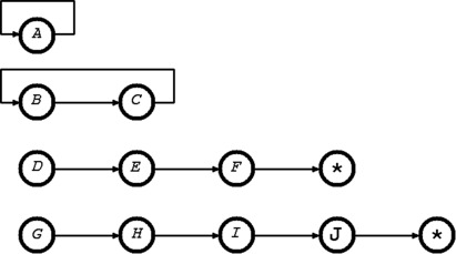
Example of corecursion for numbers

The notation $[x_1\mapsto{v_1},\ldots,x_k\mapsto{v_k}]$ denotes the function $\theta$ with domain $\{x_1,\ldots,x_k\}$ defined by $\theta(x_i)=v_i$. Using this notation, consider the Peano coalgebra $({{{\mathcal C}}},{isz},{p})$ where:

$~~~\begin{array}{ll} {{{\mathcal C}}} &= ~~~\{{{\scriptsize{A,B,C,D,E,F,G,H,I,J}}}\},\\ {isz} &= ~~~[{{\scriptsize{F\mapsto{\ast},J\mapsto{\ast}}}}],\\ {p} &= ~~~[{{\scriptsize{A\mapsto{A},B\mapsto{C},C\mapsto{B},D\mapsto{E},E\mapsto{F}, G\mapsto{H},H\mapsto{I},I\mapsto{J}}}}]. \end{array}$

${{\small\mathsf{Dom}}}({isz}) = \{{{\scriptsize{F,J}}}\}$ and ${{\small\mathsf{Dom}}}({p}) = \{{{\scriptsize{A,B,C,D,E,G,H,I}}}\}$, so ${{\small\mathsf{Dom}}}({isz})$ and ${{\small\mathsf{Dom}}}({p})$ partition ${{\mathcal C}}$.

This coalgebra is diagrammed below: an arrow from $x$ to $x'$ means that if $x\in{{\small\mathsf{Dom}}}({p})$ then ${p}(x)=x'$, and if $x\in{{\small\mathsf{Dom}}}({isz})$ then ${isz}(x)={\ast}$.

Consider now the definition of $g:{{{\mathcal C}}}{{\;{\to}\;}}{{\overline{{{\Bbb N}}}}}$ specified for $x\in{{{\mathcal C}}}$ by $g(x)={{{\mathtt{if}}}~{isz}(x){{\,{=}\,}}{\ast}~{{\mathtt{then}}}~0~{{\mathtt{else}}}~g({p}(x)){+}1}$.

Rewriting $g({{\scriptsize{A}}})$ with this equation yields:

$\begin{array}{l} g({{\scriptsize{A}}}) = g({p}({{\scriptsize{A}}})){+}1 = g({{\scriptsize{A}}}){+}1 \end{array}$

The only way this can be satisfied is with $g({{\scriptsize{A}}})=\infty$.

Rewriting $g({{\scriptsize{B}}})$ and $g({{\scriptsize{C}}})$ yields:

$\begin{array}{l} g({{\scriptsize{B}}}) = g({p}({{\scriptsize{B}}})){+}1 = g({{\scriptsize{C}}}){+}1 = (g({p}({{\scriptsize{C}}})){+}1){+}1 = (g({{\scriptsize{B}}}){+}1){+}1 = g({{\scriptsize{B}}}){+}2\\ g({{\scriptsize{C}}}) = g({p}({{\scriptsize{C}}})){+}1 = g({{\scriptsize{B}}}){+}1 = (g({p}({{\scriptsize{B}}})){+}1){+}1 = (g({{\scriptsize{C}}}){+}1){+}1 = g({{\scriptsize{C}}}){+}2 \end{array}$

The only way these can be satisfied is with $g({{\scriptsize{B}}})=\infty$ and $g({{\scriptsize{C}}})=\infty$.

Thus if $x\in\{{{\scriptsize{A}}},{{\scriptsize{B}}},{{\scriptsize{C}}}\}$ then evaluating $g(x)$ by rewriting with the equation for $g$ loops.

On other arguments the rewriting terminates:

$\begin{array}{l} g({{\scriptsize{F}}}) = 0\\ g({{\scriptsize{E}}}) = g({p}({{\scriptsize{E}}})){+}1 = g({{\scriptsize{F}}}){+}1 = 0{+}1 = 1\\ g({{\scriptsize{D}}}) = g({p}({{\scriptsize{D}}})){+}1 = g({{\scriptsize{E}}}){+}1 = 1{+}1 = 2 \end{array}$

$\begin{array}{l} g({{\scriptsize{J}}}) = 0\\ g({{\scriptsize{I}}}) = g({p}({{\scriptsize{I}}})){+}1 = g({{\scriptsize{J}}}){+}1 = 0{+}1 = 1\\ g({{\scriptsize{H}}}) = g({p}({{\scriptsize{H}}})){+}1 = g({{\scriptsize{I}}}){+}1 = 1{+}1 = 2\\ g({{\scriptsize{G}}}) = g({p}({{\scriptsize{G}}})){+}1 = g({{\scriptsize{H}}}){+}1 = 2{+}1 = 3 \end{array}$

These rewriting calculations show that:

$g=[{{\scriptsize{A\mapsto{{\normalsize{\infty}}},B\mapsto{{\normalsize{\infty}}},C\mapsto{{\normalsize{\infty}}}, D\mapsto{{\normalsize{2}}},E\mapsto{{\normalsize{1}}},F\mapsto{{\normalsize{0}}},G\mapsto{{\normalsize{3}}}, H\mapsto{{\normalsize{2}}},I\mapsto{{\normalsize{1}}},J\mapsto{{\normalsize{0}}}}}}]$

For an arbitrary Peano coalgebra $({{{\mathcal C}}},{isz},{p})$, the function $g:{{{\mathcal C}}}{{\;{\to}\;}}{{\overline{{{\Bbb N}}}}}$ satisfying the equation $~g(x)={{{\mathtt{if}}}~{isz}(x){{\,{=}\,}}{\ast}~{{\mathtt{then}}}~0~{{\mathtt{else}}}~g({p}(x)){+}1}~$ is described by:

$g(x) = \begin{cases} \! n \,\,\,\, \exists x_0\cdots x_n.~ x{{\,{=}\,}}x_0 ~\wedge~ {isz}(x_n){{\,{=}\,}}{\ast}~\wedge~ \forall i{<}n.\, p(x_i){{\,{=}\,}}x_{i{+}1} \cr \! \infty \text{ otherwise} \end{cases}$

The example just given illustrates this.

Lists and colists

If ${{\small\mathfrak{A}}}$ is a set – “${{\small\mathfrak{A}}}$” for “alphabet” – then the set ${{{\Bbb L}}_{{{\small\mathfrak{A}}}}}$ of finite lists (or strings) of members of ${{{\small\mathfrak{A}}}}$ is defined by two constructors: the empty list ${{\mathsf{nil}}}\in {{{\Bbb L}}_{{{\small\mathfrak{A}}}}}$ and the function ${{\mathsf{cons}}}:{{{\small\mathfrak{A}}}}{\times}{{{\Bbb L}}_{{{\small\mathfrak{A}}}}}{{\;{\to}\;}}{{{\Bbb L}}_{{{\small\mathfrak{A}}}}}$ which constructs the new list ${{\mathsf{cons}}}({{\mathfrak{a}}},l)$ that results from adding the element ${{\mathfrak{a}}}\in {{{\small\mathfrak{A}}}}$ to the front of list $l\in {{{\Bbb L}}_{{{\small\mathfrak{A}}}}}$.

Peano-style axioms for lists are:

${{\mathsf{nil}}}\in {{{\Bbb L}}_{{{\small\mathfrak{A}}}}}$
$\forall {{\mathfrak{a}}}\in {{{\small\mathfrak{A}}}}.~\forall l\in {{{\Bbb L}}_{{{\small\mathfrak{A}}}}}.~ {{\mathsf{cons}}}({{\mathfrak{a}}},l)\in {{{\Bbb L}}_{{{\small\mathfrak{A}}}}}$
$\forall {{\mathfrak{a}}}\in {{{\small\mathfrak{A}}}}.~\forall l\in {{{\Bbb L}}_{{{\small\mathfrak{A}}}}}.~ {{\mathsf{cons}}}({{\mathfrak{a}}},l)\neq {{\mathsf{nil}}}$
$\forall {{\mathfrak{a}}}_1\,{{\mathfrak{a}}}_2\in {{{\small\mathfrak{A}}}}.~\forall l_1\,l_2\in {{{\Bbb L}}_{{{\small\mathfrak{A}}}}}.~ {{\mathsf{cons}}}({{\mathfrak{a}}}_1,l_1){{\,{=}\,}}{{\mathsf{cons}}}({{\mathfrak{a}}}_2,l_2) {\;\Rightarrow\;}{{\mathfrak{a}}}_1{{\,{=}\,}}{{\mathfrak{a}}}_2 \wedge l_1{{\,{=}\,}}l_2$
$\forall M.~ {{\mathsf{nil}}}\in M \wedge (\forall {{\mathfrak{a}}}\in {{{\small\mathfrak{A}}}}.~\forall l\in M.~{{\mathsf{cons}}}({{\mathfrak{a}}},l)\in M) {\;\Rightarrow\;}{{{\Bbb L}}_{{{\small\mathfrak{A}}}}}\subseteq M$

Axiom 5 entails that if $l\in {{{\Bbb L}}_{{{\small\mathfrak{A}}}}}$ then $l{{\,{=}\,}}{{\mathsf{nil}}}$ or $l{{\,{=}\,}}{{\mathsf{cons}}}({{\mathfrak{a}}},l')$ for some ${{\mathfrak{a}}}\in {{{\small\mathfrak{A}}}}$ and $l'\in {{{\Bbb L}}_{{{\small\mathfrak{A}}}}}$ (to see this specialise $M$ to $\{l\mid l{{\,{=}\,}}{{\mathsf{nil}}}\vee \exists {{\mathfrak{a}}}\in {{{\small\mathfrak{A}}}}.\,\exists l'\in {{{\Bbb L}}_{{{\small\mathfrak{A}}}}}.\,l{{\,{=}\,}}{{\mathsf{cons}}}({{\mathfrak{a}}},l')\}$). This and Axiom 4 shows that there are destructors ${{\mathsf{hd}}}:{{{\Bbb L}}_{{{\small\mathfrak{A}}}}}{\;\nrightarrow\;}{{{\small\mathfrak{A}}}}$ and ${{\mathsf{tl}}}:{{{\Bbb L}}_{{{\small\mathfrak{A}}}}}{\;\nrightarrow\;}{{{\Bbb L}}_{{{\small\mathfrak{A}}}}}$, which satisfy $\forall l\in {{{\Bbb L}}_{{{\small\mathfrak{A}}}}}.~l{{\,{=}\,}}{{\mathsf{nil}}}\vee l{{\,{=}\,}}{{\mathsf{cons}}}({{\mathsf{hd}}}(l),{{\mathsf{tl}}}(l))$.

These five Peano-style axioms for lists are equivalent to the single property that if ${{\mathcal A}}$ is a set, $nl\in {{\mathcal A}}$ and $cs:{{{\small\mathfrak{A}}}}{\times}{{\mathcal A}}{{\;{\to}\;}}{{\mathcal A}}$, then there is a unique function $f:{{{\Bbb L}}_{{{\small\mathfrak{A}}}}}{{\;{\to}\;}}{{\mathcal A}}$ such that $\forall l\in {{{\Bbb L}}_{{{\small\mathfrak{A}}}}}.~f(l)={{{\mathtt{if}}}~l{{\,{=}\,}}{{\mathsf{nil}}}~{{\mathtt{then}}}~nl~{{\mathtt{else}}}~cs({{\mathsf{hd}}}(l),f({{\mathsf{tl}}}(l)))}$.

A structure $({{\mathcal A}},nl,cs)$ where $nl\in {{\mathcal A}}$ and $cs:{{{\small\mathfrak{A}}}}{\times}{{\mathcal A}}{{\;{\to}\;}}{{\mathcal A}}$ is an ${{{\small\mathfrak{A}}}}$-list algebra. The dual concept is an ${{{\small\mathfrak{A}}}}$-list coalgebra $({{\mathcal C}},test,dest)$ where ${{\mathcal C}}$ is the carrier set and $test:{{{\mathcal C}}}{\;\nrightarrow\;}\{{\ast}\}$ and $dest:{{{\mathcal C}}}{\;\nrightarrow\;}{{{\small\mathfrak{A}}}}{\times}{{{\mathcal C}}}$ are destructors whose domains partition the carrier ${{\mathcal C}}$.

Some notation is useful when discussing the dual of the ${{{\small\mathfrak{A}}}}$-list algebra $({{{\Bbb L}}_{{{\small\mathfrak{A}}}}},{{\mathsf{nil}}},{{\mathsf{cons}}})$.

For any sets $X_1$, $X_2$, if $(x_1,x_2)\in X_1{\times}{X_2}$ then ${\pi_1}(x_1,x_2){\,{=}\,}x_1$ and ${\pi_2}(x_1,x_2){\,{=}\,}x_2$. The functions ${\pi_1}:X_1{\times}{X_2}{{\;{\to}\;}}X_1$ and ${\pi_2}:X_1{\times}{X_2}{{\;{\to}\;}}X_2$ are called projections.
If $\theta_1:X_1{{\;{\to}\;}}Y_1$ and $\theta_2:X_2{{\;{\to}\;}}Y_2$, then $\theta_1{\times}{\theta_2}:X_1{\times}X_2{{\;{\to}\;}}Y_1{\times}Y_2$ is defined by $(\theta_1{\times}\theta_2)(x_1,x_2){\,{=}\,}(\theta_1(x_1),\theta_2(x_2))$. The function $\theta_1{\times}{\theta_2}$ is called the product of functions $\theta_1$ and $\theta_2$. Note that $(\theta_1{\times}\theta_2)(x){\,{=}\,}(\theta_1({\pi_1}(x)),\theta_2({\pi_2}(x)))$.
If $E$ is an expression containing a variable $n$ (e.g. $E = \sigma(n{+}1)$), then $\lambda n. E$ denotes the function that when applied to an argument returns the value obtained by evaluating $E$ after the argument has been substituted for $n$, so $\lambda n.\,\sigma(n{+}1)$ denotes the function $n \mapsto \sigma(n{+}1)$.
The identity function is denoted by ${\mathsf{id}}$, so $\forall x.\,{\mathsf{id}}(x){\,{=}\,}x$ and ${\mathsf{id}}{\,{=}\,}\lambda x.\,x$. The notation ${\mathsf{id}}_X$ is used to make the domain of ${\mathsf{id}}$ explicit, so ${\mathsf{id}}_X : X{{\;{\to}\;}}X$.

The dual of the ${{{\small\mathfrak{A}}}}$-list algebra $({{{\Bbb L}}_{{{\small\mathfrak{A}}}}},{{\mathsf{nil}}},{{\mathsf{cons}}})$ is the ${{{\small\mathfrak{A}}}}$-list coalgebra $({{{\overline{{{\Bbb L}}}}}_{{{\small\mathfrak{A}}}}},{{\mathsf{null}}},{{\mathsf{destcons}}})$ with the property that for any ${{\small\mathfrak{A}}}$-list coalgebra $({{\mathcal C}},test,dest)$, there is exactly one function $g:{{{\mathcal C}}}{{\;{\to}\;}}{{{\overline{{{\Bbb L}}}}}_{{{\small\mathfrak{A}}}}}$ such that for all $x\in{{\mathcal C}}$:

if $x\in{{\small\mathsf{Dom}}}(test)$ then
$g(x)\in{{\small\mathsf{Dom}}}({{\mathsf{null}}})$ and ${{\mathsf{null}}}(g(x))=test(x)$;
if $x\in{{\small\mathsf{Dom}}}(dest)$ then
$g(x)\in{{\small\mathsf{Dom}}}({{\mathsf{destcons}}})$ and ${{\mathsf{destcons}}}(g(x))=({\mathsf{id}}{\times}{g})(dest(x))$.

It turns out that the unique existence of $g$ determines the ${{\small\mathfrak{A}}}$-list coalgebra $({{{\overline{{{\Bbb L}}}}}_{{{\small\mathfrak{A}}}}},{{\mathsf{null}}},{{\mathsf{destcons}}})$ to have carrier set ${{{\overline{{{\Bbb L}}}}}_{{{\small\mathfrak{A}}}}}= {{{\Bbb L}}_{{{\small\mathfrak{A}}}}}\cup{{{\small\mathfrak{A}}}^{{{\Bbb N}}}}$, where ${{{\small\mathfrak{A}}}^{{{\Bbb N}}}}$ is the set of infinite lists of members of ${{\small\mathfrak{A}}}$. Formally ${{{\small\mathfrak{A}}}^{{{\Bbb N}}}}= \{\sigma\mid \sigma:{{\Bbb N}}{{\;{\to}\;}}{{\small\mathfrak{A}}}\}$, i.e. infinite lists are represented as functions $\sigma$ from the natural numbers to ${{\small\mathfrak{A}}}$, with $\sigma(n)$ being the $n^{\mathrm{th}}$ element of the list $\sigma$, counting from $0$, so $\sigma(0)$ is the first element. The nullary destructor ${{\mathsf{null}}}:\{{{\mathsf{nil}}}\}{{\;{\to}\;}}\{{\ast}\}$ satisfies ${{{\mathsf{null}}}}({{\mathsf{nil}}}){{\,{=}\,}}{\ast}$ and the unary destructor ${{\mathsf{destcons}}}:\{l\mid l\neq{{\mathsf{nil}}}\}{{\;{\to}\;}}{{{\overline{{{\Bbb L}}}}}_{{{\small\mathfrak{A}}}}}$ is the function that returns the pair $({{\mathsf{hd}}}(l),{{\mathsf{tl}}}(l))$ when applied to a non-empty finite list $l$, and returns the pair $(\sigma(0),\lambda n.\,\sigma(n{+}1))$ when applied to an infinite list $\sigma$.

It is useful to extend ${{\mathsf{cons}}}$, ${{\mathsf{hd}}}$ and ${{\mathsf{tl}}}$ from ${{\Bbb L}}_{\alpha}$ to all of ${{{\Bbb L}}_{{{\small\mathfrak{A}}}}}\cup{{{\small\mathfrak{A}}}^{{{\Bbb N}}}}$ by defining:

$\begin{array}{ll} {{\mathsf{cons}}}({{\mathfrak{a}}},\sigma) &\!\!\!\!\!= ~\lambda n.\,{{{\mathtt{if}}}~n{{\,{=}\,}}0~{{\mathtt{then}}}~{{\mathfrak{a}}}~{{\mathtt{else}}}~\sigma(n{-}1)}\\ {{\mathsf{hd}}}(\sigma) &\!\!\!\!\!= ~\sigma(0)\\ {{\mathsf{tl}}}(\sigma) &\!\!\!\!\!= ~\lambda n.\,\sigma(n{+}1)) \end{array}$

With these definitions, the unique function $g:{{\mathcal C}}{{\;{\to}\;}}{{{\overline{{{\Bbb L}}}}}_{{{\small\mathfrak{A}}}}}$ is defined by the single equation:

$g(x)~=~{{{\mathtt{if}}}~test(x){{\,{=}\,}}{\ast}~{{\mathtt{then}}}~{{\mathsf{nil}}}~{{\mathtt{else}}}~{{\mathsf{cons}}}(({\mathsf{id}}{\times}{g})(dest(x)))}$

which can also be written as:

$g(x)~=~{{{\mathtt{if}}}~test(x){{\,{=}\,}}{\ast}~{{\mathtt{then}}}~{{\mathsf{nil}}}~{{\mathtt{else}}}~{{\mathsf{cons}}}({\pi_1}(dest(x)),g({\pi_2}(dest(x))))}$

and is equivalent to:

${{\mathsf{null}}}(g(x)){{\,{=}\,}}test(x) ~\wedge~{{\mathsf{hd}}}(g(x)){{\,{=}\,}}({\pi_1}(dest(x)) ~\wedge~{{\mathsf{tl}}}(g(x)){{\,{=}\,}}g({\pi_2}(dest(x)))$

Note the ways in which colists are dual to lists:

constructors ${{\mathsf{nil}}}\in{{{\Bbb L}}_{{{\small\mathfrak{A}}}}}$, ${{\mathsf{cons}}}:{{\small\mathfrak{A}}}{\times}{{{\Bbb L}}_{{{\small\mathfrak{A}}}}}{{\;{\to}\;}}{{{\Bbb L}}_{{{\small\mathfrak{A}}}}}$ versus
destructors$\phantom{s}$ ${{\mathsf{null}}}:{{{\overline{{{\Bbb L}}}}}_{{{\small\mathfrak{A}}}}}{\;\nrightarrow\;}\{{\ast}\}$, ${{\mathsf{destcons}}}:{{{\overline{{{\Bbb L}}}}}_{{{\small\mathfrak{A}}}}}{\;\nrightarrow\;}{{\small\mathfrak{A}}}{\times}{{{\overline{{{\Bbb L}}}}}_{{{\small\mathfrak{A}}}}}$;
unique $f:{{{\Bbb L}}_{{{\small\mathfrak{A}}}}}{{\;{\to}\;}}{{\mathcal A}}$ versus
unique $g:{{\mathcal C}}{{\;{\to}\;}}{{{\overline{{{\Bbb L}}}}}_{{{\small\mathfrak{A}}}}}$;
define $f$ on constructors: $f({{\mathsf{nil}}}){\,{=}\,}nl \wedge f({{\mathsf{cons}}}({{\mathfrak{a}}},l)){\,{=}\,}cs({{\mathfrak{a}}},f(l))$ versus
define destructors on $g$: ${{\mathsf{null}}}(g(x)){=}test(x)\,{\wedge}\,{{\mathsf{destcons}}}(g(x)){=}({\mathsf{id}}{{\times}}{g})(dest(x))\mathrm{;}$
recursion$\phantom{co}$ $f(l)={{{\mathtt{if}}}~l{{\,{=}\,}}{{\mathsf{nil}}}~{{\mathtt{then}}}~nl~{{\mathtt{else}}}~cs({{\mathsf{hd}}}(l),f({{\mathsf{tl}}}(l)))}$ versus
corecursion $g(x)={{{\mathtt{if}}}~test(x){{\,{=}\,}}{\ast}~{{\mathtt{then}}}~{{\mathsf{nil}}}~{{\mathtt{else}}}~{{\mathsf{cons}}}(({\mathsf{id}}{\times}{g})(dest(x)))}$.
recursion always terminates versus
corecursion sometimes doesn’t terminate (see example below).

Example of corecursion for lists

The Peano coalgebra example used above can be reinterpreted as a ${{{\overline{{{\Bbb L}}}}}_{{{\small\mathfrak{A}}}}}$ coalgebra.

$\begin{array}{ll} {{{\small\mathfrak{A}}}}&\!\!\!\!\!=\!\!\!\!\! ~~\{{{\scriptsize{A,B,C,D,E,F,G,H,I,J}}}\},\\ {{{\mathcal C}}} &\!\!\!\!\!\!=\!\!\!\! ~~\{{{\scriptsize{A,B,C,D,E,F,G,H,I,J}}}\},\\ {test} &\!\!\!\!\!\!=\!\!\!\! ~~[{{\scriptsize{F\,{\mapsto}\,{\ast},J\,{\mapsto}\,{\ast}}}}],\\ {dest} &\!\!\!\!\!\!=\!\!\!\! ~~[{{\scriptsize{A\,{\mapsto}\,{(A,A)},B\,{\mapsto}\,{(B,C)},C\,{\mapsto}\,{(C,B)}, D\,{\mapsto}\,{(D,E)},E\,{\mapsto}\,{(E,F)},}}}\\ &\!\!\!\!\!\!\phantom{=}\!\!\!\! ~~~ {{\scriptsize{G\,{\mapsto}\,{(G,H)}, H\,{\mapsto}\,{(H,I)},I\,{\mapsto}\,{(I,J)}}}}]. \end{array}$

${{\small\mathsf{Dom}}}({test}) = \{{{\scriptsize{F,J}}}\}$ and ${{\small\mathsf{Dom}}}({dest}) = \{{{\scriptsize{A,B,C,D,E,G,H,I}}}\}$, so ${{\small\mathsf{Dom}}}(test)$ and ${{\small\mathsf{Dom}}}(dest)$ partition ${{\mathcal C}}$.

In the diagram below: an arrow from $x$ to $x'$ means that if $x\in{{\small\mathsf{Dom}}}(dest)$ then ${dest}(x)=(x,x')$, and if $x\in{{\small\mathsf{Dom}}}({test})$ then ${test}(x)={\ast}$.

Consider now the definition of $g:{{{\mathcal C}}}{{\;{\to}\;}}{{{\overline{{{\Bbb L}}}}}_{{{\small\mathfrak{A}}}}}$ specified for $x\in{{{\mathcal C}}}$ by $g(x)~=~{{{\mathtt{if}}}~test(x){{\,{=}\,}}{\ast}~{{\mathtt{then}}}~{{\mathsf{nil}}}~{{\mathtt{else}}}~{{\mathsf{cons}}}(({\mathsf{id}}{\times}{g})(dest(x)))}$.

The notation ${\mathbf{\small{[}}}{{\mathfrak{a}}}_0,{{\mathfrak{a}}}_1,\ldots,{{\mathfrak{a}}}_n{\mathbf{\small{]}}}$ abbreviates ${{\mathsf{cons}}}({{\mathfrak{a}}}_0,{{\mathsf{cons}}}({{\mathfrak{a}}}_1,\ldots,{{\mathsf{cons}}}({{\mathfrak{a}}}_n,{{\mathsf{nil}}})\cdots))$ and ${\mathbf{\small{[}}}\;{\mathbf{\small{]}}}$ is used as a synonym for ${{\mathsf{nil}}}$.

Rewriting $g({{\scriptsize{A}}})$ with the equation defining $g$ yields:

$\begin{array}{l} g({{\scriptsize{A}}}) = {{\mathsf{cons}}}(({\mathsf{id}}{\times}{g})(dest({{\scriptsize{A}}}))) = {{\mathsf{cons}}}(({\mathsf{id}}{\times}{g})({{\scriptsize{A}}},{{\scriptsize{A}}})) = {{\mathsf{cons}}}({{\scriptsize{A}}},g({{\scriptsize{A}}})) = {\mathbf{\small{[}}}{{\scriptsize{A}}},g({{\scriptsize{A}}}){\mathbf{\small{]}}}\end{array}$

The only way this can be satisfied is with $g({{\scriptsize{A}}})$ being the infinite list of ${{\scriptsize{A}}}$s, i.e. $g({{\scriptsize{A}}}) = {\mathbf{\small{[}}}{{\scriptsize{A,A,A,\ldots}}}{\mathbf{\small{]}}}$. Formally this is the function $\lambda n.\,{{\scriptsize{A}}}$.

Rewriting $g({{\scriptsize{B}}})$ and $g({{\scriptsize{C}}})$ yields:

\(\begin{array}{l} g({{\scriptsize{B}}}) = {{\mathsf{cons}}}(({\mathsf{id}}{\times}{g})(dest({{\scriptsize{B}}})))\\ \phantom{g({{\scriptsize{B}}})} = {{\mathsf{cons}}}(({\mathsf{id}}{\times}{g})({{\scriptsize{B}}},{{\scriptsize{C}}}))\\ \phantom{g({{\scriptsize{B}}})} = {{\mathsf{cons}}}({{\scriptsize{B}}},g({{\scriptsize{C}}}))\\ \phantom{g({{\scriptsize{B}}})} = {{\mathsf{cons}}}({{\scriptsize{B}}},{{\mathsf{cons}}}(({\mathsf{id}}{\times}{g})(dest({{\scriptsize{C}}}))))\\ \phantom{g({{\scriptsize{B}}})} = {{\mathsf{cons}}}({{\scriptsize{B}}},{{\mathsf{cons}}}({{\scriptsize{C}}},g({{\scriptsize{B}}})))\\ \phantom{g({{\scriptsize{B}}})} = {\mathbf{\small{[}}}{{\scriptsize{B}}},{{\scriptsize{C}}},g({{\scriptsize{B}}}){\mathbf{\small{]}}}\\ g({{\scriptsize{C}}}) = {{\mathsf{cons}}}(({\mathsf{id}}{\times}{g})(dest({{\scriptsize{C}}})))\\ \phantom{g({{\scriptsize{C}}})} = {{\mathsf{cons}}}(({\mathsf{id}}{\times}{g})({{\scriptsize{C}}},{{\scriptsize{B}}}))\\ \phantom{g({{\scriptsize{C}}})} = {{\mathsf{cons}}}({{\scriptsize{C}}},g({{\scriptsize{B}}}))\\ \phantom{g({{\scriptsize{C}}})} = {{\mathsf{cons}}}({{\scriptsize{C}}},{{\mathsf{cons}}}(({\mathsf{id}}{\times}{g})(dest({{\scriptsize{B}}}))))\\ \phantom{g({{\scriptsize{C}}})} = {{\mathsf{cons}}}({{\scriptsize{C}}},{{\mathsf{cons}}}({{\scriptsize{B}}},g({{\scriptsize{C}}})))\\ \phantom{g({{\scriptsize{C}}})} = {\mathbf{\small{[}}}{{\scriptsize{C}}},{{\scriptsize{B}}},g({{\scriptsize{C}}}){\mathbf{\small{]}}}\end{array}\)

The only way these can be satisfied is with $g({{\scriptsize{B}}})$ being the infinite list that repeats ${{\scriptsize{B}}}$ followed by ${{\scriptsize{C}}}$, i.e. $g({{\scriptsize{B}}}) = {\mathbf{\small{[}}}{{\scriptsize{B,C,B,C,B,C,B,C\ldots}}}{\mathbf{\small{]}}}$ and $g({{\scriptsize{C}}})$ being the infinite list that repeats ${{\scriptsize{C}}}$ followed by ${{\scriptsize{B}}}$, i.e. $g({{\scriptsize{C}}}) = {\mathbf{\small{[}}}{{\scriptsize{C,B,C,B,C,B,C,B\ldots}}}{\mathbf{\small{]}}}$.

Thus if $x\in\{{{\scriptsize{A}}},{{\scriptsize{B}}},{{\scriptsize{C}}}\}$, then evaluating $g(x)$ by rewriting with the equation for $g$ returns an infinite list, i.e. a member of ${{{\small\mathfrak{A}}}^{{{\Bbb N}}}}$.

On other arguments the rewriting results in a finite list, i.e. a member of ${{{\Bbb L}}_{{{\small\mathfrak{A}}}}}$. The rewriting calculations below take bigger steps than the ones above (the expansion of $({\mathsf{id}}{\times}{g})({\cdots})$ is omitted).

$\begin{array}{l} g({{\scriptsize{F}}}) = {{\mathsf{nil}}}= {\mathbf{\small{[}}}\;{\mathbf{\small{]}}}\\ g({{\scriptsize{E}}}) = {{\mathsf{cons}}}({{\scriptsize{E}}}, g({{\scriptsize{F}}})) = {{\mathsf{cons}}}({{\scriptsize{E}}}, {{\mathsf{nil}}}) = {\mathbf{\small{[}}}{{\scriptsize{E}}}{\mathbf{\small{]}}}\\ g({{\scriptsize{D}}}) = {{\mathsf{cons}}}({{\scriptsize{D}}}, g({{\scriptsize{E}}})) = {{\mathsf{cons}}}({{\scriptsize{D}}}, {\mathbf{\small{[}}}{{\scriptsize{E}}}{\mathbf{\small{]}}}) = {\mathbf{\small{[}}}{{\scriptsize{D,E}}}{\mathbf{\small{]}}}\end{array}$

$\begin{array}{l} g({{\scriptsize{J}}}) = {{\mathsf{nil}}}= {\mathbf{\small{[}}}\;{\mathbf{\small{]}}}\\ g({{\scriptsize{I}}}) = {{\mathsf{cons}}}({{\scriptsize{I}}}, g({{\scriptsize{J}}})) = {{\mathsf{cons}}}({{\scriptsize{I}}}, {{\mathsf{nil}}}) = {\mathbf{\small{[}}}{{\scriptsize{I}}}{\mathbf{\small{]}}}\\ g({{\scriptsize{H}}}) = {{\mathsf{cons}}}({{\scriptsize{H}}}, g({{\scriptsize{I}}})) = {{\mathsf{cons}}}({{\scriptsize{H}}}, {\mathbf{\small{[}}}{{\scriptsize{I}}}{\mathbf{\small{]}}}) = {\mathbf{\small{[}}}{{\scriptsize{H,I}}}{\mathbf{\small{]}}}\\ g({{\scriptsize{G}}}) = {{\mathsf{cons}}}({{\scriptsize{G}}}, g({{\scriptsize{H}}})) = {{\mathsf{cons}}}({{\scriptsize{G}}}, {\mathbf{\small{[}}}{{\scriptsize{H,I}}}{\mathbf{\small{]}}}) = {\mathbf{\small{[}}}{{\scriptsize{G,H,I}}}{\mathbf{\small{]}}}\end{array}$

These rewriting calculations show that:

$\begin{array}{l} g= [{{\scriptsize{A\,{\mapsto}\,{\mathbf{\small{[}}}A,A,A,\ldots{\mathbf{\small{]}}}}}},\, {{\scriptsize{B\,{\mapsto}\,{\mathbf{\small{[}}}B,C,B,C,B,C,B,C,\ldots{\mathbf{\small{]}}}}}},\, {{\scriptsize{C\,{\mapsto}\,{\mathbf{\small{[}}}C,B,C,B,C,B,C,B,\ldots{\mathbf{\small{]}}}}}}, \\ \phantom{g=[\,} {{\scriptsize{D\,{\mapsto}\,{\mathbf{\small{[}}}D,E{\mathbf{\small{]}}}}}},\, {{\scriptsize{E\,{\mapsto}\,{\mathbf{\small{[}}}E{\mathbf{\small{]}}}}}},\, {{\scriptsize{F\,{\mapsto}\,{\mathbf{\small{[}}}\;{\mathbf{\small{]}}}}}},\, {{\scriptsize{G\,{\mapsto}\,{\mathbf{\small{[}}}G,H,I{\mathbf{\small{]}}}}}},\, {{\scriptsize{H\,{\mapsto}\,{\mathbf{\small{[}}}H,I{\mathbf{\small{]}}}}}},\, {{\scriptsize{I\,{\mapsto}\,{\mathbf{\small{[}}}I{\mathbf{\small{]}}}}}},\, {{\scriptsize{J\,{\mapsto}\,{\mathbf{\small{[}}}\;{\mathbf{\small{]}}}}}}] \end{array}$

For an arbitrary ${{\small\mathfrak{A}}}$-list coalgebra $({{\mathcal C}},test,dest)$, the function $g:{{\mathcal C}}{{\;{\to}\;}}{{{\overline{{{\Bbb L}}}}}_{{{\small\mathfrak{A}}}}}$ satisfying the equation $g(x)~=~{{{\mathtt{if}}}~test(x){{\,{=}\,}}{\ast}~{{\mathtt{then}}}~{{\mathsf{nil}}}~{{\mathtt{else}}}~{{\mathsf{cons}}}(({\mathsf{id}}{\times}{g})(dest(x)))}$ is described by:

$g(x) = \begin{cases} \! {\mathbf{\small{[}}}{{\mathfrak{a}}}_0,\ldots, {{\mathfrak{a}}}_{n{-}1}\,{\mathbf{\small{]}}}\,\, \exists x_0\cdots x_{n}.\, \cr \phantom{\! {\mathbf{\small{[}}}{{\mathfrak{a}}}_0,\ldots, {{\mathfrak{a}}}_{n{-}1}{\mathbf{\small{]}}}\,\,\,\, \exists} x{{\,{=}\,}}x_0 ~\wedge~ test(x_{n}){{\,{=}\,}}{\ast}~\wedge~ \forall i{<}n.\, dest(x_i){{\,{=}\,}}({{\mathfrak{a}}}_i,x_{i{+}1}) \cr \cr \! {\mathbf{\small{[}}}{{\mathfrak{a}}}_0,{{\mathfrak{a}}}_1,{{\mathfrak{a}}}_2,\ldots{\mathbf{\small{]}}}\, \exists \sigma:{{\Bbb N}}{{\;{\to}\;}}{{\mathcal C}}.\; x{{\,{=}\,}}\sigma(0) ~\wedge~ \forall i.\, dest(\sigma(i)){{\,{=}\,}}({{\mathfrak{a}}}_i,\sigma(i{+}1)) \end{cases}$

The example just given illustrates this.

Coinduction and bisimulation

Induction for natural numbers is the fifth Peano axiom. For lists, it is the fifth of the Peano-like axioms given at the start of the section on Lists and colists above. Both of these are equivalent to the uniqueness of the functions resulting from the principle of recursive definition from ${{\Bbb N}}$ or ${{\Bbb L}}_{\alpha}$ to the carriers of the appropriate algebras.

As far as I can discover there is no canonical notion of coinduction for the dual of natural numbers or lists. The term “coinduction” (actually “co-induction”) is generally attributed to Milner and Tofte in their 1991 paper Co-induction in relational semantics whose abstract is:

An application of the mathematical theory of maximum fixed points of monotonic set operators to relational semantics is presented. It is shown how an important proof method which we call co-induction, a variant of Park’s (1969) principle of fixpoint induction, can be used to prove the consistency of the static and the dynamic relational semantics of a small functional programming language with recursive functions.

Milner and Tofte’s paper is based on fixed points, but other more recent work on coinduction is based on terminal algebras, which is the approach taken here (see the sections below entitled least and greatest fixed points and Initial and terminal algebras).

The coinduction principle described here is called bisimulation coinduction, where a bisimulation is a relation $R$ between members of the carrier of a coalgebra. The name “bisimulation coinduction” is not standard, usually just called “coinduction” is used. The principle is derived from the corecursion equation defining the unique functions from arbitrary coalgebras to the conumber coalgebra ${{\overline{{{\Bbb N}}}}}$ or to the colist coalgebra ${{\overline{{{\Bbb L}}}}}_{\alpha}$. This derivation is given for conumbers and colists in the sections on the justification of bisimulation coinduction for numbers and the justification of bisimulation coinduction for lists.

Bisimulation coinduction for conumbers

For the conatural numbers ${{\overline{{{\Bbb N}}}}}$, a bisimulation is a relation $R\subseteq {{\overline{{{\Bbb N}}}}}{\times}{{\overline{{{\Bbb N}}}}}$ such that if $(n_1,n_2)\in R$ then either $n_1{{\,{=}\,}}0$ and $n_2{\,{=}\,}0$ or else $n_1{\,{=}\,}{{\small\mathsf{S}}}(n_1')$ and $n_2{\,{=}\,}{{\small\mathsf{S}}}(n_2')$ for some $(n_1',n_2')\in R$.

The bisimulation coinduction principle for ${{\overline{{{\Bbb N}}}}}$ states that if $R$ is any bisimulation, then $R \subseteq \{(n,n)\mid n \in {{\overline{{{\Bbb N}}}}}\}$.

Example of bisimulation coinduction for numbers

It’s hard to come up with examples for ${{\overline{{{\Bbb N}}}}}$ that illustrate useful applications of coinduction. This is because coinduction is actually not much use in practice. The rather contrived example that follows is inspired by part of a (hopefully) more convincing example used later to illustrate coinduction on lists. In the example ${\mathsf{even}}(n)$ means that $n$ is an even number (${\mathsf{even}}(0)$ is considered true) and ${\mathsf{odd}}(n)$ that $n$ is odd.

Consider the unique function $g:{{\Bbb N}}{{\;{\to}\;}}{{\overline{{{\Bbb N}}}}}$ determined by the Peano coalgebra $({{\Bbb N}},isz,p)$ where ${{\small\mathsf{Dom}}}(isz) = \{n\mid {\mathsf{even}}(n)\}$ and ${{\small\mathsf{Dom}}}(p) = \{n \mid {\mathsf{odd}}(n)\}$, and the destructors are defined by $p(n)={\ast}{\;\Leftrightarrow\;}{\mathsf{even}}(n)$ and $s(n)=n{+}2$. This function $g$ is defined by:

$g(x)={{{\mathtt{if}}}~isz(x){{\,{=}\,}}{\ast}~{{\mathtt{then}}}~0~{{\mathtt{else}}}~g(p(x)){+}1}$

and with the particular $isz$ and $p$ just specified, is equivalent to:

$g(n) = {{{\mathtt{if}}}~{\mathsf{even}}(n)~{{\mathtt{then}}}~0~{{\mathtt{else}}}~g(n{+}2){+}1}$

Intuitively this function returns $0$ on even numbers and loops on odd numbers, so is equal to $h:{{\Bbb N}}{{\;{\to}\;}}{{\overline{{{\Bbb N}}}}}$ defined by: $h(n) = {{{\mathtt{if}}}~{\mathsf{even}}(n)~{{\mathtt{then}}}~0~{{\mathtt{else}}}~\infty}$.

This can be proved by showing that $R = \{(g(n),h(n))\mid n\in{{\Bbb N}}\}$ is a bisimulation.

Suppose $(n_1,n_2)\in R$, then $n_1=g(n)$ and $n_2=h(n)$ for some $n\in{{\Bbb N}}$.

If $n$ is even then $n_1 {\,{=}\,}g(n) {\,{=}\,}0$ and $n_2 {\,{=}\,}h(n) {\,{=}\,}0$.

If $n$ is not even, then $n_1 {\,{=}\,}g(n){\,{=}\,}g(n{+}2){+}1{\,{=}\,}{{\small\mathsf{S}}}(g(n{+}2))$ (including when $g(n{+}2){\,{=}\,}\infty$) and $n_2{\,{=}\,}h(n){\,{=}\,}\infty{\,{=}\,}{{\small\mathsf{S}}}(\infty){\,{=}\,}{{\small\mathsf{S}}}(h(n{+}2))$, as $n{+}2$ is not even if $n$ is not even.

Thus if $(n_1,n_2)\in R$ then either $n_1{{\,{=}\,}}0$ and $n_2{\,{=}\,}0$ or else $n_1{\,{=}\,}{{\small\mathsf{S}}}(n_1')$ and $n_2{\,{=}\,}{{\small\mathsf{S}}}(n_2')$ for some $(n_1',n_2')\in R$ – here $n_1'{\,{=}\,}g(n{+}2)$ and $n_2'{\,{=}\,}h(n{+}2)$ – so $R$ is a bisimulation, hence by the bisimulation coinduction principle it follows that $\forall n\in{{\Bbb N}}.\,g(n) {\,{=}\,}h(n)$.

Justification of bisimulation coinduction for numbers

To establish that the uniqueness of corecursively specified functions entails the principle of bisimulation coinduction, let $R\subseteq {{\overline{{{\Bbb N}}}}}{\times}{{\overline{{{\Bbb N}}}}}$ be a bisimulation. Consider the Peano coalgebra $(R,isz_R,p_R)$, where $isz_R(n_1,n_2){\,{=}\,}{\ast}{\;\Leftrightarrow\;}n_1{{\,{=}\,}}0\wedge n_2{{\,{=}\,}}0$ and $p_R(n_1,n_2){\,{=}\,}({{\small\mathsf{P}}}(n_1),{{\small\mathsf{P}}}(n_2))$. The definition of a bisimulation ensures that the domains of $isz_R$ and $p_R$ partition the coalgebra carrier set $R$. By the defining property of $({{\overline{{{\Bbb N}}}}},{{\mathsf{is}0}},{{\small\mathsf{P}}})$, there is a unique function $g:R{{\;{\to}\;}}{{\overline{{{\Bbb N}}}}}$ such that for all $(n_1,n_2)\in R$:

$g(n_1,n_2)={{{\mathtt{if}}}~isz_R(n_1,n_2){{\,{=}\,}}{\ast}~{{\mathtt{then}}}~0~{{\mathtt{else}}}~g(p_R(n_1,n_2)){+}1}$

i.e. for all $(n_1,n_2)\in R$:

$g(n_1,n_2)={{{\mathtt{if}}}~n_1{{\,{=}\,}}0\wedge n_2{{\,{=}\,}}0~{{\mathtt{then}}}~0~{{\mathtt{else}}}~g({{\small\mathsf{P}}}(n_1),{{\small\mathsf{P}}}(n_2)){+}1}$

Recall the projection functions: ${\pi_1}(\sigma_1,\sigma_2){\,{=}\,}\sigma_1$ and ${\pi_2}(\sigma_1,\sigma_2){\,{=}\,}\sigma_2$. As is about to be shown, it is easy to verify the equation for $g$ is satisfied with both $g={\pi_1}$ and $g={\pi_2}$.

Taking $g={\pi_1}$ and assuming $(n_1,n_2)\in R$:

${\pi_1}(n_1,n_2)={{{\mathtt{if}}}~n_1{{\,{=}\,}}0\wedge n_2{{\,{=}\,}}0~{{\mathtt{then}}}~0~{{\mathtt{else}}}~{\pi_1}({{\small\mathsf{P}}}(n_1),{{\small\mathsf{P}}}(n_2)){+}1}$

which simplifies to:

$n_1={{{\mathtt{if}}}~n_1{{\,{=}\,}}0\wedge n_2{{\,{=}\,}}0~{{\mathtt{then}}}~0~{{\mathtt{else}}}~{{\small\mathsf{P}}}(n_1){+}1}$

which holds for all $(n_1,n_2)\in R$, since if $(n_1,n_2)\in R$ then $n_1{\,{=}\,}0 {\;\Leftrightarrow\;}n_2{\,{=}\,}0$ as $R$ is a bisimulation.

Now take $g={\pi_2}$, then assuming $(n_1,n_2)\in R$:

${\pi_2}(n_1,n_2)={{{\mathtt{if}}}~n_1{{\,{=}\,}}0\wedge n_2{{\,{=}\,}}0~{{\mathtt{then}}}~0~{{\mathtt{else}}}~{\pi_2}({{\small\mathsf{P}}}(n_1),{{\small\mathsf{P}}}(n_2)){+}1}$

which simplifies to:

$n_2={{{\mathtt{if}}}~n_1{{\,{=}\,}}0\wedge n_2{{\,{=}\,}}0~{{\mathtt{then}}}~0~{{\mathtt{else}}}~{{\small\mathsf{P}}}(n_2){+}1}$

which also holds for all $(n_1,n_2)\in R$.

Since $g$ is unique, ${\pi_1}:R{{\;{\to}\;}}{{\overline{{{\Bbb N}}}}}$ and ${\pi_2}:R{{\;{\to}\;}}{{\overline{{{\Bbb N}}}}}$ must be the same function, so if $(n_1,n_2)\in R$ then $n_1={\pi_1}(n_1,n_2)={\pi_2}(n_1,n_2)=n_2$, so $R\subseteq\{(n,n)\mid \in{{\overline{{{\Bbb N}}}}}\}$.

The argument just given shows that the bisimulation coinduction principle follows from the uniqueness of the function $g:{{\mathcal C}}{{\;{\to}\;}}{{\overline{{{\Bbb N}}}}}$ corecursively specified by:

$g(x)={{{\mathtt{if}}}~isz(x){{\,{=}\,}}{\ast}~{{\mathtt{then}}}~0~{{\mathtt{else}}}~g(p(x)){+}1}$

To prove the reverse implication, i.e. that the bisimulation coinduction principle entails the uniqueness of corecursively specified functions, suppose that:

$\begin{array}{l} g_1(x)={{{\mathtt{if}}}~isz(x){\,{=}\,}{\ast}~{{\mathtt{then}}}~0~{{\mathtt{else}}}~g_1(p(x)){+}1}\\ g_2(x)={{{\mathtt{if}}}~isz(x){\,{=}\,}{\ast}~{{\mathtt{then}}}~0~{{\mathtt{else}}}~g_2(p(x)){+}1} \end{array}$

then it’s easy to see that $R$, where $R = \{(g_1(x),g_2(x)) \mid x \in {{\mathcal C}}\}$, is a bisimulation.

If $(n_1,n_2)\in R$ then $n_1 {\,{=}\,}g_1(x)$ and $n_2 {\,{=}\,}g_2(x)$ for some $x\in {{\mathcal C}}$.

If $isz(x){\,{=}\,}{\ast}$, then $n_1 {\,{=}\,}g_1(x) {\,{=}\,}0$ and $n_2 {\,{=}\,}g_2(x) {\,{=}\,}0$.

If $isz(x)\neq{\ast}$, then $n_1 {\,{=}\,}g_1(x) {\,{=}\,}g_1(p(x)){+}1{\,{=}\,}{{\small\mathsf{S}}}(g_1(p(x)))$ and $n_2 {\,{=}\,}g_2(x) {\,{=}\,}g_2(p(x)){+}1{\,{=}\,}{{\small\mathsf{S}}}(g_2(p(x)))$. Since $(g_1(p(x)),g_2(p(x)))\in R$ by the definition of $R$, it follows that $R$ is a bisimulation, hence by the bisimulation coinduction principle: $\forall x\in{{\mathcal C}}.\,g_1(x) {\,{=}\,}g_2(x)$.

Bisimulation coinduction for lists

A bisimulation on ${{{\overline{{{\Bbb L}}}}}_{{{\small\mathfrak{A}}}}}$ is a relation $R\subseteq {{{\overline{{{\Bbb L}}}}}_{{{\small\mathfrak{A}}}}}{\times}{{{\overline{{{\Bbb L}}}}}_{{{\small\mathfrak{A}}}}}$ such that if $(\sigma_1,\sigma_2)\in R$ then either $\sigma_1{\,{=}\,}{{\mathsf{nil}}}$ and $\sigma_2{\,{=}\,}{{\mathsf{nil}}}$ or else $\sigma_1{\,{=}\,}{{\mathsf{cons}}}({{\mathfrak{a}}},\sigma_1')$ and $\sigma_2{\,{=}\,}{{\mathsf{cons}}}({{\mathfrak{a}}},\sigma_2')$ for some ${{\mathfrak{a}}}\in{{\small\mathfrak{A}}}$ and $(\sigma_1',\sigma_2')\in R$.

The bisimulation coinduction principle for ${{{\overline{{{\Bbb L}}}}}_{{{\small\mathfrak{A}}}}}$ states that if $R$ is any bisimulation, then $R \subseteq \{(\sigma,\sigma)\mid \sigma \in {{{\overline{{{\Bbb L}}}}}_{{{\small\mathfrak{A}}}}}\}$.

Examples of bisimulation coinduction for lists

Recall the corecursively defined functions ${{\small\mathsf{CountFrom}}}$, ${{\small\mathsf{CountUp}}}$ and ${{\small\mathsf{CountUpTo}}}$ from the summary at the beginning of this article.

It is asserted in the summary that $R_1$ and $R_2$ are bisimulations, where:

This assertion is verified in the next two paragraphs.

Suppose $(\sigma_1,\sigma_2)\in R_1$, then $\sigma_1{\,{=}\,}{{\small\mathsf{CountUp}}}(m,n)$ and $\sigma_2{\,{=}\,}{{\small\mathsf{CountFrom}}}(m)$ for some $(m,n)$ with $m>n$. It follows from the definitions of ${{\small\mathsf{CountUp}}}$ and ${{\small\mathsf{CountFrom}}}$ that $\sigma_1{\,{=}\,}{{\mathsf{cons}}}(m,{{\small\mathsf{CountUp}}}(m{+}1,n))$ and $\sigma_2{\,{=}\,}{{\mathsf{cons}}}(m,{{\small\mathsf{CountFrom}}}(m{+}1))$. As $m>n$ implies $m{+}1>n$, it follows that $({{\small\mathsf{CountUp}}}(m{+}1,n),{{\small\mathsf{CountFrom}}}(m{+}1))\in R_1$, hence $R_1$ is a bisimulation, so by bisimulation coinduction: $\forall m\,n\in{{\Bbb N}}.\, m>n {\;\Rightarrow\;}{{\small\mathsf{CountUp}}}(m,n){\,{=}\,}{{\small\mathsf{CountFrom}}}(m)$.

Suppose $(\sigma_1,\sigma_2)\in R_2$, then $\sigma_1{\,{=}\,}{{\small\mathsf{CountUp}}}(m,n)$ and $\sigma_2{\,{=}\,}{{\small\mathsf{CountUpTo}}}(m,n)$ for some $(m,n)$ with $m\leq n$. If $m{\,{=}\,}n$ then from the definitions of ${{\small\mathsf{CountUp}}}$ and ${{\small\mathsf{CountUpTo}}}$ it follows that $\sigma_1{\,{=}\,}{{\mathsf{nil}}}$ and $\sigma_2{\,{=}\,}{{\mathsf{nil}}}$. If $m<n$, then from the definitions of ${{\small\mathsf{CountUp}}}$ and ${{\small\mathsf{CountUpTo}}}$ it follows that $\sigma_1{\,{=}\,}{{\mathsf{cons}}}(m,{{\small\mathsf{CountUp}}}(m{+}1,n))$ and $\sigma_2{\,{=}\,}{{\mathsf{cons}}}(m,{{\small\mathsf{CountUpTo}}}(m{+}1,n))$. As $m<n$ implies $m{+}1\leq n$, it follows that $({{\small\mathsf{CountUp}}}(m{+}1,n), {{\small\mathsf{CountUpTo}}}(m{+}1,n))\in R_2$, hence $R_2$ is a bisimulation, so by bisimulation coinduction: $\forall m\,n\in{{\Bbb N}}.\, m\leq n {\;\Rightarrow\;}{{\small\mathsf{CountUp}}}(m,n){\,{=}\,}{{\small\mathsf{CountUpTo}}}(m,n)$.

By combining the results of coinduction based on the bisimulations $R_1$ and $R_2$, the equation below can be deduced.

${{\small\mathsf{CountUp}}}(m,n) = {{{\mathtt{if}}}~m\leq n~{{\mathtt{then}}}~{{\small\mathsf{CountUpTo}}}(m,n)~{{\mathtt{else}}}~{{\small\mathsf{CountFrom}}}(m)}$

The remaining examples in this section are adapted from similar ones in An introduction to (co)algebra and (co)induction by Bart Jacobs and Jan Rutten, except that here lists can be finite or infinite, but in Jacobs & Rutton they are only infinite. Allowing lists to be finite complicates the examples as there are extra cases to consider. It’s not clear whether the examples below illustrate anything significant that isn’t already shown by the examples above.

If $\sigma\in{{{\overline{{{\Bbb L}}}}}_{{{\small\mathfrak{A}}}}}$ – i.e. $\sigma$ is a finite or infinite list – then $g_{{\mathsf{even}}}(\sigma)$ is the sublist consisting of those elements at even numbered positions and $g_{{\mathsf{odd}}}(\sigma)$ is the sublist consisting of those elements at odd numbered positions.

$\begin{array}{llllllllllllll} \sigma: & {{\mathfrak{a}}}_0 & {{\mathfrak{a}}}_1 & {{\mathfrak{a}}}_2 & {{\mathfrak{a}}}_3 & {{\mathfrak{a}}}_4 & {{\mathfrak{a}}}_5 & {{\mathfrak{a}}}_6 & {{\mathfrak{a}}}_7 & {{\mathfrak{a}}}_8 & {{\mathfrak{a}}}_9 & {{\mathfrak{a}}}_{10} & {{\mathfrak{a}}}_{11} & \cdots\\ g_{{\mathsf{even}}}(\sigma): & {{\mathfrak{a}}}_0 & & {{\mathfrak{a}}}_2 & & {{\mathfrak{a}}}_4 & & {{\mathfrak{a}}}_6 & & {{\mathfrak{a}}}_8 & & {{\mathfrak{a}}}_{10} & & \cdots\\ g_{{\mathsf{odd}}}(\sigma): & & {{\mathfrak{a}}}_1 & & {{\mathfrak{a}}}_3 & & {{\mathfrak{a}}}_5 & & {{\mathfrak{a}}}_7 & & {{\mathfrak{a}}}_9 & & {{\mathfrak{a}}}_{11} & \cdots \end{array}$

The functions $g_{{\mathsf{even}}}$ and $g_{{\mathsf{odd}}}$ are defined by corecursion below, and then two lemmas are proved by bisumulation coinduction:

Lemma 1. $\forall \sigma\in{{{\overline{{{\Bbb L}}}}}_{{{\small\mathfrak{A}}}}}.\,g_{{\mathsf{odd}}}(\sigma) = g_{{\mathsf{even}}}({{\mathsf{tl}}}(\sigma))$

Lemma 2. $\forall\sigma\in{{{\overline{{{\Bbb L}}}}}_{{{\small\mathfrak{A}}}}}.\,\sigma\neq{{\mathsf{nil}}}{\;\Rightarrow\;}{{\mathsf{tl}}}(g_{{\mathsf{even}}}(\sigma)){\,{=}\,}g_{{\mathsf{odd}}}({{\mathsf{tl}}}(\sigma))$

Next ${{\mathsf{merge}}}(\sigma_1,\sigma_2)$ is defined by corecursion to be the interleaving of $\sigma_1$ and $\sigma_2$. Using these two lemmas, it is then shown by bisimulation coinduction that ${{\mathsf{merge}}}(g_{{\mathsf{even}}}(\sigma),g_{{\mathsf{odd}}}(\sigma)){\,{=}\,}\sigma$.

To define $g_{{\mathsf{even}}}$ and $g_{{\mathsf{odd}}}$ consider the following ${{\small\mathfrak{A}}}$-list coalgebras:

$\begin{array}{ll} {\Bbb C}_{{\mathsf{even}}}&\!\!\!\!\!= ({{{\overline{{{\Bbb L}}}}}_{{{\small\mathfrak{A}}}}},~{{\mathsf{test}}}_{{\mathsf{even}}},~{{\mathsf{dest}}}_{{\mathsf{even}}})\\ {\Bbb C}_{{\mathsf{odd}}}&\!\!\!\!\!= ({{{\overline{{{\Bbb L}}}}}_{{{\small\mathfrak{A}}}}},~{{\mathsf{test}}}_{{\mathsf{odd}}},~{{\mathsf{dest}}}_{{\mathsf{odd}}}) \end{array}$

where

$\begin{array}{ll} {{\mathsf{test}}}_{{\mathsf{even}}}(\sigma){\,{=}\,}{\ast}&\!\!\!\!\! {\;\Leftrightarrow\;}~ \sigma{\,{=}\,}{{\mathsf{nil}}}\\ {{\mathsf{test}}}_{{\mathsf{odd}}}(\sigma)\;{\,{=}\,}{\ast}&\!\!\!\!\! {\;\Leftrightarrow\;}~ \sigma{\,{=}\,}{{\mathsf{nil}}}~\text{or}~ {{\mathsf{tl}}}(\sigma){\,{=}\,}{{\mathsf{nil}}}\end{array}$

and

$\begin{array}{ll} {{\mathsf{dest}}}_{{\mathsf{even}}}(\sigma) &\!\!\!\!\! =~ ({{\mathsf{hd}}}(\sigma),~ {{{\mathtt{if}}}~{{\mathsf{tl}}}(\sigma){\,{=}\,}{{\mathsf{nil}}}~{{\mathtt{then}}}~{{\mathsf{nil}}}~{{\mathtt{else}}}~{{\mathsf{tl}}}({{\mathsf{tl}}}(\sigma))}) \\ {{\mathsf{dest}}}_{{\mathsf{odd}}}(\sigma) &\!\!\!\!\! =~ ({{\mathsf{hd}}}({{\mathsf{tl}}}(\sigma)),~ {{\mathsf{tl}}}({{\mathsf{tl}}}(\sigma))) \\ \end{array}$

The domains of destructors partition ${\Bbb C}_{{\mathsf{even}}}$, so the definition of ${{\mathsf{test}}}_{{\mathsf{even}}}$ entails that the domain of ${{\mathsf{dest}}}_{{\mathsf{even}}}$ is the set of lists with at least one element. The definitions of ${{\mathsf{dest}}}_{{\mathsf{even}}}$ is illustrated by:

$\begin{array}{l} {{\mathsf{dest}}}_{{\mathsf{even}}}({\mathbf{\small{[}}}{{\mathfrak{a}}}_0{\mathbf{\small{]}}}){\,{=}\,}({{\mathfrak{a}}}_0, {{\mathsf{nil}}})\\ {{\mathsf{dest}}}_{{\mathsf{even}}}({\mathbf{\small{[}}}{{\mathfrak{a}}}_0,{{\mathfrak{a}}}_1{\mathbf{\small{]}}}){\,{=}\,}({{\mathfrak{a}}}_0, {{\mathsf{nil}}})\\ {{\mathsf{dest}}}_{{\mathsf{even}}}({\mathbf{\small{[}}}{{\mathfrak{a}}}_0,{{\mathfrak{a}}}_1,{{\mathfrak{a}}}_2{\mathbf{\small{]}}}){\,{=}\,}({{\mathfrak{a}}}_0, {\mathbf{\small{[}}}{{\mathfrak{a}}}_2{\mathbf{\small{]}}})\\ {{\mathsf{dest}}}_{{\mathsf{even}}}({\mathbf{\small{[}}}{{\mathfrak{a}}}_0,{{\mathfrak{a}}}_1,{{\mathfrak{a}}}_2,{{\mathfrak{a}}}_3,\ldots{\mathbf{\small{]}}}){\,{=}\,}({{\mathfrak{a}}}_0, {\mathbf{\small{[}}}{{\mathfrak{a}}}_2,{{\mathfrak{a}}}_3,\ldots{\mathbf{\small{]}}}) \end{array}$

The domains of destructors partition ${\Bbb C}_{{\mathsf{odd}}}$, so the definition of ${{\mathsf{test}}}_{{\mathsf{odd}}}$ entails that the domain of ${{\mathsf{dest}}}_{{\mathsf{odd}}}$ is the set of lists with at least two elements. The definition of ${{\mathsf{dest}}}_{{\mathsf{odd}}}$ is illustrated by:

$\begin{array}{l} {{\mathsf{dest}}}_{{\mathsf{odd}}}({\mathbf{\small{[}}}{{\mathfrak{a}}}_0,{{\mathfrak{a}}}_1{\mathbf{\small{]}}}) {\,{=}\,}({{\mathfrak{a}}}_1, {{\mathsf{nil}}})\\ {{\mathsf{dest}}}_{{\mathsf{odd}}}({\mathbf{\small{[}}}{{\mathfrak{a}}}_0,{{\mathfrak{a}}}_1,{{\mathfrak{a}}}_2{\mathbf{\small{]}}}) {\,{=}\,}({{\mathfrak{a}}}_1, {\mathbf{\small{[}}}{{\mathfrak{a}}}_2{\mathbf{\small{]}}})\\ {{\mathsf{dest}}}_{{\mathsf{odd}}}({\mathbf{\small{[}}}{{\mathfrak{a}}}_0,{{\mathfrak{a}}}_1,{{\mathfrak{a}}}_2,{{\mathfrak{a}}}_3,\ldots{\mathbf{\small{]}}}) {\,{=}\,}({{\mathfrak{a}}}_1, {\mathbf{\small{[}}}{{\mathfrak{a}}}_2,{{\mathfrak{a}}}_3,\ldots{\mathbf{\small{]}}})\\ \end{array}$

Recall the general form of the unique corecursively specified function

$g:{{\mathcal C}}\to{{{\overline{{{\Bbb L}}}}}_{{{\small\mathfrak{A}}}}}$ from the carrier of a coalgebra $({{\mathcal C}},test,dest)$ to the carrier of $({{{\overline{{{\Bbb L}}}}}_{{{\small\mathfrak{A}}}}},{{\mathsf{null}}},{{\mathsf{destcons}}})$:

$g(x)~=~{{{\mathtt{if}}}~test(x){{\,{=}\,}}{\ast}~{{\mathtt{then}}}~{{\mathsf{nil}}}~{{\mathtt{else}}}~{{\mathsf{cons}}}(({\mathsf{id}}{\times}{g})(dest(x)))}$

For the coalgebras ${\Bbb C}_{{\mathsf{even}}}$ and ${\Bbb C}_{{\mathsf{odd}}}$, this general schema instantiates, respectively, to:

$\begin{array}{l} g_{{\mathsf{even}}}(\sigma) = ~\mathtt{if}~{\sigma{\,{=}\,}{{\mathsf{nil}}}}\\ \phantom{g_{{\mathsf{even}}}(\sigma) = ~~} ~\mathtt{then}~ {{{\mathsf{nil}}}}\\ \phantom{g_{{\mathsf{even}}}(\sigma) = ~~} ~\mathtt{else}~ {{{\mathsf{cons}}}({{\mathsf{hd}}}(\sigma), g_{{\mathsf{even}}}({{{\mathtt{if}}}~{{\mathsf{tl}}}(\sigma){\,{=}\,}{{\mathsf{nil}}}~{{\mathtt{then}}}~{{\mathsf{nil}}}~{{\mathtt{else}}}~{{\mathsf{tl}}}({{\mathsf{tl}}}(\sigma))))}}\\ \\ g_{{\mathsf{odd}}}(\sigma) = ~\mathtt{if}~{\sigma{\,{=}\,}{{\mathsf{nil}}}~\text{or}~ {{\mathsf{tl}}}(\sigma){\,{=}\,}{{\mathsf{nil}}}}\\ \phantom{g_{{\mathsf{odd}}}(\sigma) = ~~} ~\mathtt{then}~{{{\mathsf{nil}}}}\\ \phantom{g_{{\mathsf{odd}}}(\sigma) = ~~} ~\mathtt{else}~ {{{\mathsf{cons}}}({{\mathsf{hd}}}({{\mathsf{tl}}}(\sigma)), g_{{\mathsf{odd}}}({{\mathsf{tl}}}({{\mathsf{tl}}}(\sigma)))} \end{array}$

These equations look intuitively correct.

To prove Lemma 1: $\forall \sigma\in{{{\overline{{{\Bbb L}}}}}_{{{\small\mathfrak{A}}}}}.\,g_{{\mathsf{odd}}}(\sigma) {\,{=}\,}g_{{\mathsf{even}}}({{\mathsf{tl}}}(\sigma))$, let $R=\{(g_{{\mathsf{odd}}}(\sigma),g_{{\mathsf{even}}}({{\mathsf{tl}}}(\sigma)))\mid\sigma\in{{{\overline{{{\Bbb L}}}}}_{{{\small\mathfrak{A}}}}}\}$. It is shown below that $R$ is a bisimulation.

If $(\sigma_1,\sigma_2)\in R$, then $\sigma_1{\,{=}\,}g_{{\mathsf{odd}}}(\sigma)$ and $\sigma_2{\,{=}\,}g_{{\mathsf{even}}}({{\mathsf{tl}}}(\sigma))$ for some $\sigma\in{{{\overline{{{\Bbb L}}}}}_{{{\small\mathfrak{A}}}}}$. Three cases need to be considered.

If $\sigma{{\,{=}\,}}{{\mathsf{nil}}}$ or ${{\mathsf{tl}}}(\sigma){{\,{=}\,}}{{\mathsf{nil}}}$ then $\sigma_1{{\,{=}\,}}\sigma_2{{\,{=}\,}}{{\mathsf{nil}}}$ by the definitions of $g_{{\mathsf{even}}}$ and $g_{{\mathsf{odd}}}$.
If $\sigma\neq{{\mathsf{nil}}}$ and ${{\mathsf{tl}}}(\sigma)\neq{{\mathsf{nil}}}$ and ${{\mathsf{tl}}}({{\mathsf{tl}}}(\sigma){\,{=}\,}{{\mathsf{nil}}}$ then $\sigma_1{{\,{=}\,}}g_{{\mathsf{odd}}}(\sigma){{\,{=}\,}}{{\mathsf{cons}}}({{\mathsf{hd}}}({{\mathsf{tl}}}(\sigma)),g_{{\mathsf{odd}}}({{\mathsf{nil}}}))$ and $\sigma_2{{\,{=}\,}}g_{{\mathsf{even}}}({{\mathsf{tl}}}(\sigma)){{\,{=}\,}}{{\mathsf{cons}}}({{\mathsf{hd}}}({{\mathsf{tl}}}(\sigma)) g_{{\mathsf{even}}}({{\mathsf{nil}}}))$. As $g_{{\mathsf{odd}}}({{\mathsf{nil}}}){\,{=}\,}{{\mathsf{nil}}}$ and $g_{{\mathsf{even}}}({{\mathsf{nil}}}){\,{=}\,}{{\mathsf{nil}}}$, $(g_{{\mathsf{odd}}}({{\mathsf{nil}}}),g_{{\mathsf{even}}}({{\mathsf{nil}}}))\in R$.
If $\sigma\neq{{\mathsf{nil}}}$ and ${{\mathsf{tl}}}(\sigma)\neq{{\mathsf{nil}}}$ and ${{\mathsf{tl}}}({{\mathsf{tl}}}(\sigma)\neq{{\mathsf{nil}}}$ then $\sigma_1{{\,{=}\,}}g_{{\mathsf{odd}}}(\sigma){{\,{=}\,}}{{\mathsf{cons}}}({{\mathsf{hd}}}({{\mathsf{tl}}}(\sigma)), g_{{\mathsf{odd}}}({{\mathsf{tl}}}({{\mathsf{tl}}}(\sigma))))$ and $\sigma_2{{\,{=}\,}}g_{{\mathsf{even}}}({{\mathsf{tl}}}(\sigma)){{\,{=}\,}}{{\mathsf{cons}}}({{\mathsf{hd}}}({{\mathsf{tl}}}(\sigma)), g_{{\mathsf{even}}}({{\mathsf{tl}}}({{\mathsf{tl}}}({{\mathsf{tl}}}(\sigma)))))$. Thus $({{\mathsf{tl}}}(\sigma_1), {{\mathsf{tl}}}(\sigma_2)){\,{=}\,}(g_{{\mathsf{odd}}}({{\mathsf{tl}}}({{\mathsf{tl}}}(\sigma))),g_{{\mathsf{even}}}({{\mathsf{tl}}}({{\mathsf{tl}}}({{\mathsf{tl}}}(\sigma))))) \in R$.

As $(\sigma_1,\sigma_2)\in R$ if either $\sigma_1{\,{=}\,}{{\mathsf{nil}}}$ and $\sigma_2{\,{=}\,}{{\mathsf{nil}}}$ or else $\sigma_1{\,{=}\,}{{\mathsf{cons}}}({{\mathfrak{a}}},\sigma_1')$ and $\sigma_2{\,{=}\,}{{\mathsf{cons}}}({{\mathfrak{a}}},\sigma_2')$ for some ${{\mathfrak{a}}}\in{{\small\mathfrak{A}}}$ and $(\sigma_1',\sigma_2')\in R$, it follows that $R$ is a bisimulation.

To prove Lemma 2: $\sigma\neq{{\mathsf{nil}}}{\;\Rightarrow\;}{{\mathsf{tl}}}(g_{{\mathsf{even}}}(\sigma)){\,{=}\,}g_{{\mathsf{odd}}}({{\mathsf{tl}}}(\sigma))$, let $R=\{({{\mathsf{tl}}}(g_{{\mathsf{even}}}(\sigma)), g_{{\mathsf{odd}}}({{\mathsf{tl}}}(\sigma))\mid\sigma\in{{{\overline{{{\Bbb L}}}}}_{{{\small\mathfrak{A}}}}}\wedge \sigma\neq{{\mathsf{nil}}}\}$. It is shown below that $R$ is a bisimulation.

If $(\sigma_1,\sigma_2)\in R$, then $\sigma_1{\,{=}\,}{{\mathsf{tl}}}(g_{{\mathsf{even}}}(\sigma))$ and $\sigma_2{\,{=}\,}g_{{\mathsf{odd}}}({{\mathsf{tl}}}(\sigma))$ for some $\sigma\neq{{\mathsf{nil}}}$. Three cases need to be considered.

If ${{\mathsf{tl}}}(\sigma){\,{=}\,}{{\mathsf{nil}}}$ then $\sigma_1{\,{=}\,}\sigma_2{\,{=}\,}{{\mathsf{nil}}}$ by the definitions of $g_{{\mathsf{even}}}$ and $g_{{\mathsf{odd}}}$.
If ${{\mathsf{tl}}}(\sigma)\neq{{\mathsf{nil}}}$ and ${{\mathsf{tl}}}({{\mathsf{tl}}}(\sigma)){\,{=}\,}{{\mathsf{nil}}}$ then $\sigma_1{\,{=}\,}{{\mathsf{tl}}}(g_{{\mathsf{even}}}(\sigma)){{\,{=}\,}}g_{{\mathsf{even}}}({{\mathsf{tl}}}({{\mathsf{tl}}}(\sigma))){\,{=}\,}{{\mathsf{nil}}}$ and $\sigma_2{{\,{=}\,}}g_{{\mathsf{odd}}}({{\mathsf{tl}}}(\sigma)){\,{=}\,}{{\mathsf{nil}}}$ by the definitions of $g_{{\mathsf{even}}}$ and $g_{{\mathsf{odd}}}$.
If ${{\mathsf{tl}}}(\sigma)\neq{{\mathsf{nil}}}$ and ${{\mathsf{tl}}}(\sigma)\neq{{\mathsf{nil}}}$ and ${{\mathsf{tl}}}({{\mathsf{tl}}}(\sigma))\neq{{\mathsf{nil}}}$ then $\sigma_1{\,{=}\,}{{\mathsf{tl}}}(g_{{\mathsf{even}}}(\sigma)) {\,{=}\,}g_{{\mathsf{even}}}({{\mathsf{tl}}}({{\mathsf{tl}}}(\sigma))) {\,{=}\,}{{\mathsf{cons}}}({{\mathsf{hd}}}({{\mathsf{tl}}}({{\mathsf{tl}}}(\sigma))),{{\mathsf{tl}}}(g_{{\mathsf{even}}}({{\mathsf{tl}}}({{\mathsf{tl}}}(\sigma)))))$ and $\sigma_2{{\,{=}\,}}g_{{\mathsf{odd}}}({{\mathsf{tl}}}(\sigma)){\,{=}\,}{{\mathsf{cons}}}({{\mathsf{hd}}}({{\mathsf{tl}}}({{\mathsf{tl}}}(\sigma))), g_{{\mathsf{odd}}}({{\mathsf{tl}}}({{\mathsf{tl}}}({{\mathsf{tl}}}(\sigma)))))$. As
${{\mathsf{tl}}}({{\mathsf{tl}}}(\sigma))\neq{{\mathsf{nil}}}$, $({{\mathsf{tl}}}(\sigma_1), {{\mathsf{tl}}}(\sigma_2)){\,{=}\,}({{\mathsf{tl}}}(g_{{\mathsf{even}}}({{\mathsf{tl}}}({{\mathsf{tl}}}(\sigma)))), g_{{\mathsf{odd}}}({{\mathsf{tl}}}({{\mathsf{tl}}}({{\mathsf{tl}}}(\sigma))))) \in R$.

The function ${{\mathsf{merge}}}:{{{\overline{{{\Bbb L}}}}}_{{{\small\mathfrak{A}}}}}{\times}{{{\overline{{{\Bbb L}}}}}_{{{\small\mathfrak{A}}}}}{{\;{\to}\;}}{{{\overline{{{\Bbb L}}}}}_{{{\small\mathfrak{A}}}}}$ interleaves two lists. It will be proved by bisimulation coinduction that $\forall \sigma\in{{{\overline{{{\Bbb L}}}}}_{{{\small\mathfrak{A}}}}}.\,{{\mathsf{merge}}}(g_{{\mathsf{even}}}(\sigma),g_{{\mathsf{odd}}}(\sigma)){\,{=}\,}\sigma$. Before proving this, the function ${{\mathsf{merge}}}$ needs to be defined. The natural recursion to achieve this is:

$\begin{array}{l} {{\mathsf{merge}}}(\sigma_1,\sigma_2) = \\ ~\mathtt{if}~ {\sigma_1{\,{=}\,}{{\mathsf{nil}}}}\\ ~~\mathtt{then}~ {\sigma_2}\\ ~~\mathtt{else}~ \\ ~~~\mathtt{if}~ {{{\mathsf{tl}}}(\sigma_1){\,{=}\,}{{\mathsf{nil}}}} \\ ~~~~\mathtt{then}~ {{{\mathsf{cons}}}({{\mathsf{hd}}}(\sigma_1),\sigma_2)} \\ ~~~~\mathtt{else}~ {{{\mathsf{cons}}}({{\mathsf{hd}}}(\sigma_1),{{\mathsf{merge}}}(\sigma_2,{{\mathsf{tl}}}(\sigma_1)))}\\ \end{array}$

To make this fit the corecursion format:

$g(x)~=~{{{\mathtt{if}}}~test(x){{\,{=}\,}}{\ast}~{{\mathtt{then}}}~{{\mathsf{nil}}}~{{\mathtt{else}}}~{{\mathsf{cons}}}(({\mathsf{id}}{\times}{g})(dest(x)))}$

where, $x$ ranges over pairs $(\sigma_1,\sigma_2)$ of lists, the destructors $test$ and $dest$ need to be defined. To achieve this the equation for ${{\mathsf{merge}}}$ can be reformulated to:

$\begin{array}{l} {{\mathsf{merge}}}(\sigma_1,\sigma_2) = \\ ~\mathtt{if}~ {\sigma_1{\,{=}\,}{{\mathsf{nil}}}}~\text{and}~\sigma_2{\,{=}\,}{{\mathsf{nil}}}\\ ~~\mathtt{then}~ {{{\mathsf{nil}}}}\\ ~~\mathtt{else}~ \\ ~~~\mathtt{if}~ {\sigma_1{\,{=}\,}{{\mathsf{nil}}}} \\ ~~~~\mathtt{then}~ {{{\mathsf{cons}}}({{\mathsf{hd}}}(\sigma_2),{{\mathsf{merge}}}(\sigma_1,{{\mathsf{tl}}}(\sigma_2))} \\ ~~~~\mathtt{else}~ {{{\mathsf{cons}}}({{\mathsf{hd}}}(\sigma_1),{{\mathsf{merge}}}(\sigma_2,{{\mathsf{tl}}}(\sigma_1)))}\\ \end{array}$

This reformulated equation is shown equivalent to the original equation below. The reformulated version becomes an instance of

$g(x)~=~{{{\mathtt{if}}}~test(x){{\,{=}\,}}{\ast}~{{\mathtt{then}}}~{{\mathsf{nil}}}~{{\mathtt{else}}}~{{\mathsf{cons}}}(({\mathsf{id}}{\times}{g})(dest(x)))}$

if $g={{\mathsf{merge}}}$ and $test:\{({{\mathsf{nil}}},{{\mathsf{nil}}})\}{{\;{\to}\;}}\{{\ast}\}$ is (necessarily) defined by:

$\begin{array}{l} test(\sigma_1,\sigma_2){\,{=}\,}{\ast}~{\;\Leftrightarrow\;}~ \sigma_1{\,{=}\,}{{\mathsf{nil}}}~\text{and}~\sigma_2{\,{=}\,}{{\mathsf{nil}}}\\ \end{array}$

and $dest:\{(\sigma_1,\sigma_2)\mid \sigma_1\neq{{\mathsf{nil}}}~\text{or}~\sigma_2\neq{{\mathsf{nil}}}\} {{\;{\to}\;}}{{\small\mathfrak{A}}}{\times}({{{\overline{{{\Bbb L}}}}}_{{{\small\mathfrak{A}}}}}{\times}{{{\overline{{{\Bbb L}}}}}_{{{\small\mathfrak{A}}}}})\;$ by:

$\begin{array}{l} dest(\sigma_1,\sigma_2) ~=~ \mathtt{if}~{\sigma_1{\,{=}\,}{{\mathsf{nil}}}} \\ \phantom{dest(\sigma_1,\sigma_2) ~= ~~} \mathtt{then}~ {({{\mathsf{hd}}}(\sigma_2),(\sigma_1,{{\mathsf{tl}}}(\sigma_2)))}\\ \phantom{dest(\sigma_1,\sigma_2) ~= ~~} \mathtt{else}~ {({{\mathsf{hd}}}(\sigma_1),(\sigma_2,{{\mathsf{tl}}}(\sigma_1)))} \end{array}$

The reformulated equation for ${{\mathsf{merge}}}$ is then the unique function from the carrier of the coalgebra $({{{\overline{{{\Bbb L}}}}}_{{{\small\mathfrak{A}}}}}{\times}{{{\overline{{{\Bbb L}}}}}_{{{\small\mathfrak{A}}}}},test,dest)$ to the carrier of the coalgebra $({{{\overline{{{\Bbb L}}}}}_{{{\small\mathfrak{A}}}}},{{\mathsf{null}}},{{\mathsf{destcons}}}).$

The original recursion for ${{\mathsf{merge}}}$ is equivalent to the reformulated equation because $\sigma_2{\,{=}\,}{{\mathsf{cons}}}({{\mathsf{hd}}}(\sigma_2),{{\mathsf{tl}}}(\sigma_2))$ and ${{\mathsf{merge}}}({{\mathsf{nil}}},{{\mathsf{tl}}}(\sigma_2)){\,{=}\,}{{\mathsf{tl}}}(\sigma_2)$, when $\sigma_2\neq{{\mathsf{nil}}}$. The second of these equations is an instance of $\forall \sigma\in{{{\overline{{{\Bbb L}}}}}_{{{\small\mathfrak{A}}}}}.\,{{\mathsf{merge}}}({{\mathsf{nil}}},\sigma){\,{=}\,}\sigma$, which is proved by bisimulation coinduction by showing that $R = \{({{\mathsf{merge}}}({{\mathsf{nil}}},\sigma),\sigma)\mid\sigma\in{{{\overline{{{\Bbb L}}}}}_{{{\small\mathfrak{A}}}}}\}$ is a bisimulation.

To show this let $(\sigma_1,\sigma_2)\in R$, then $\sigma_1{\,{=}\,}{{\mathsf{merge}}}({{\mathsf{nil}}},\sigma)$ and $\sigma_2{\,{=}\,}\sigma$ for some $\sigma\in{{{\overline{{{\Bbb L}}}}}_{{{\small\mathfrak{A}}}}}$. If $\sigma{\,{=}\,}{{\mathsf{nil}}}$, then $\sigma_1{\,{=}\,}\sigma_2{\,{=}\,}{{\mathsf{nil}}}$. If $\sigma\neq{{\mathsf{nil}}}$ then $\sigma_1{\,{=}\,}{{\mathsf{cons}}}({{\mathsf{hd}}}(\sigma),{{\mathsf{merge}}}({{\mathsf{nil}}},{{\mathsf{tl}}}(\sigma)))$ and $\sigma_2{\,{=}\,}\sigma{\,{=}\,}{{\mathsf{cons}}}({{\mathsf{hd}}}(\sigma),{{\mathsf{tl}}}(\sigma))$. Thus $({{\mathsf{tl}}}(\sigma_1),{{\mathsf{tl}}}(\sigma_2)){\,{=}\,}({{\mathsf{merge}}}({{\mathsf{nil}}},{{\mathsf{tl}}}(\sigma)),{{\mathsf{tl}}}(\sigma)) \in R$, so $R$ is a bisimulation.

To prove ${{\mathsf{merge}}}(g_{{\mathsf{even}}}(\sigma),g_{{\mathsf{odd}}}(\sigma)){\,{=}\,}\sigma$ for arbitrary $\sigma\in{{{\overline{{{\Bbb L}}}}}_{{{\small\mathfrak{A}}}}}$, it is sufficient to show that $R = \{({{\mathsf{merge}}}(g_{{\mathsf{even}}}(\sigma),g_{{\mathsf{odd}}}(\sigma)),\sigma)\mid \sigma \in {{{\overline{{{\Bbb L}}}}}_{{{\small\mathfrak{A}}}}}\}$ is a bisimulation.

If $(\sigma_1,\sigma_2)\in R$, then $\sigma_1{\,{=}\,}{{\mathsf{merge}}}(g_{{\mathsf{even}}}(\sigma),g_{{\mathsf{odd}}}(\sigma))$ and $\sigma_2{\,{=}\,}\sigma$ for some $\sigma\in{{{\overline{{{\Bbb L}}}}}_{{{\small\mathfrak{A}}}}}$. Three cases need to be considered.

If $\sigma{\,{=}\,}{{\mathsf{nil}}}$ then $\sigma_1{\,{=}\,}{{\mathsf{merge}}}({{\mathsf{nil}}},{{\mathsf{nil}}}){\,{=}\,}{{\mathsf{nil}}}$ and $\sigma_2{\,{=}\,}\sigma{\,{=}\,}{{\mathsf{nil}}}$.
If $\sigma\neq{{\mathsf{nil}}}$ and ${{\mathsf{tl}}}(\sigma){\,{=}\,}{{\mathsf{nil}}}$ then $\sigma_1{\,{=}\,}{{\mathsf{merge}}}({{\mathsf{cons}}}({{\mathsf{hd}}}(\sigma),{{\mathsf{nil}}}),{{\mathsf{nil}}}){\,{=}\,}{{\mathsf{cons}}}({{\mathsf{hd}}}(\sigma),{{\mathsf{nil}}})$ and $\sigma_2{\,{=}\,}\sigma{\,{=}\,}{{\mathsf{cons}}}({{\mathsf{hd}}}(\sigma),{{\mathsf{nil}}})$.
If $\sigma\neq{{\mathsf{nil}}}$ and ${{\mathsf{tl}}}(\sigma)\neq{{\mathsf{nil}}}$ by the definitions of $g_{{\mathsf{even}}}$, $g_{{\mathsf{odd}}}$ and ${{\mathsf{merge}}}$, and using Lemma 1 and Lemma 2:
\(\begin{array}{l} \sigma_1{\,{=}\,}{{\mathsf{merge}}}(g_{{\mathsf{even}}}(\sigma),g_{{\mathsf{odd}}}(\sigma))\\ \phantom{\sigma_1}{\,{=}\,}{{\mathsf{merge}}}({{\mathsf{cons}}}({{\mathsf{hd}}}(\sigma),g_{{\mathsf{even}}}({{\mathsf{tl}}}({{\mathsf{tl}}}(\sigma)))), {{\mathsf{cons}}}({{\mathsf{hd}}}({{\mathsf{tl}}}(\sigma)),g_{{\mathsf{odd}}}({{\mathsf{tl}}}({{\mathsf{tl}}}(\sigma)))))\\ \phantom{\sigma_1}{\,{=}\,}{{\mathsf{cons}}}({{\mathsf{hd}}}(\sigma),{{\mathsf{merge}}}({{\mathsf{cons}}}({{\mathsf{hd}}}({{\mathsf{tl}}}(\sigma)), g_{{\mathsf{odd}}}({{\mathsf{tl}}}({{\mathsf{tl}}}(\sigma)))),g_{{\mathsf{even}}}({{\mathsf{tl}}}({{\mathsf{tl}}}(\sigma)))))\\ \phantom{\sigma_1}{\,{=}\,}{{\mathsf{cons}}}({{\mathsf{hd}}}(\sigma),{{\mathsf{merge}}}({{\mathsf{cons}}}({{\mathsf{hd}}}({{\mathsf{tl}}}(\sigma)), {{\mathsf{tl}}}(g_{{\mathsf{even}}}({{\mathsf{tl}}}(\sigma)))),g_{{\mathsf{odd}}}({{\mathsf{tl}}}(\sigma))))\\ \phantom{\sigma_1}{\,{=}\,}{{\mathsf{cons}}}({{\mathsf{hd}}}(\sigma),{{\mathsf{merge}}}({{\mathsf{cons}}}({{\mathsf{hd}}}(g_{{\mathsf{even}}}({{\mathsf{tl}}}(\sigma))), {{\mathsf{tl}}}(g_{{\mathsf{even}}}({{\mathsf{tl}}}(\sigma)))),g_{{\mathsf{odd}}}({{\mathsf{tl}}}(\sigma))))\\ \phantom{\sigma_1}{\,{=}\,}{{\mathsf{cons}}}({{\mathsf{hd}}}(\sigma),{{\mathsf{merge}}}(g_{{\mathsf{even}}}({{\mathsf{tl}}}(\sigma)),g_{{\mathsf{odd}}}({{\mathsf{tl}}}(\sigma)))) \text{.} \end{array}\)
Also $\sigma_2{\,{=}\,}\sigma{\,{=}\,}{{\mathsf{cons}}}({{\mathsf{hd}}}(\sigma),{{\mathsf{tl}}}(\sigma))$, so $({{\mathsf{tl}}}(\sigma_1),{{\mathsf{tl}}}(\sigma_2)){\,{=}\,}({{\mathsf{merge}}}(g_{{\mathsf{even}}}({{\mathsf{tl}}}(\sigma)),g_{{\mathsf{odd}}}({{\mathsf{tl}}}(\sigma))),{{\mathsf{tl}}}(\sigma))\in R$. Hence $R$ is a bisimulation.

Justification of bisimulation coinduction for lists

A bisimulation on ${{{\overline{{{\Bbb L}}}}}_{{{\small\mathfrak{A}}}}}$ is a relation $R\subseteq {{{\overline{{{\Bbb L}}}}}_{{{\small\mathfrak{A}}}}}{\times}{{{\overline{{{\Bbb L}}}}}_{{{\small\mathfrak{A}}}}}$ such that $(\sigma_1,\sigma_2)\in R$ if either $\sigma_1{\,{=}\,}{{\mathsf{nil}}}$ and $\sigma_2{\,{=}\,}{{\mathsf{nil}}}$ or else $\sigma_1\neq {{\mathsf{nil}}}$ and $\sigma_2\neq {{\mathsf{nil}}}$ and ${{\mathsf{hd}}}(\sigma_1)={{\mathsf{hd}}}(\sigma_2)$ and $({{\mathsf{tl}}}(\sigma_1),{{\mathsf{tl}}}(\sigma_2))\in R$.

To establish that the uniqueness of corecursively specified functions entails the principle of bisimulation coinduction, let $R\subseteq {{{\overline{{{\Bbb L}}}}}_{{{\small\mathfrak{A}}}}}{\times}{{{\overline{{{\Bbb L}}}}}_{{{\small\mathfrak{A}}}}}$ be a bisimulation. Define the ${{\small\mathfrak{A}}}$-list coalgebra $(R,test_R,dest_R)$ by: $test_R(\sigma_1,\sigma_2){\,{=}\,}{\ast}{\;\Leftrightarrow\;}~ \sigma_1{{\,{=}\,}}{{\mathsf{nil}}}\wedge\sigma_2{{\,{=}\,}}{{\mathsf{nil}}}$ and $dest_R(\sigma_1,\sigma_2){\,{=}\,}({{\mathsf{hd}}}(\sigma_1),({{\mathsf{tl}}}(\sigma_1),{{\mathsf{tl}}}(\sigma_2)))$. Note that if $(\sigma_1,\sigma_2)\in R$ then ${{\mathsf{hd}}}(\sigma_1){\,{=}\,}{{\mathsf{hd}}}(\sigma_2)$, so in the definition of $dest_R$ in the last sentence ${{\mathsf{hd}}}(\sigma_1)$ could have been ${{\mathsf{hd}}}(\sigma_2)$.

The definition of a bisimulation ensures that the domains of $test_R$ and $dest_R$ partition the coalgebra carrier set $R$. By the defining property of $({{{\overline{{{\Bbb L}}}}}_{{{\small\mathfrak{A}}}}},{{\mathsf{null}}},{{\mathsf{destcons}}})$, there is a unique function $g:R{{\;{\to}\;}}{{{\overline{{{\Bbb L}}}}}_{{{\small\mathfrak{A}}}}}$ such that for all $(\sigma_1,\sigma_2)\in R$:

$g(\sigma_1,\sigma_2)~=~ {{{\mathtt{if}}}~test_R(\sigma_1,\sigma_2) {{\,{=}\,}}{\ast}~{{\mathtt{then}}}~{{\mathsf{nil}}}~{{\mathtt{else}}}~{{\mathsf{cons}}}(({\mathsf{id}}{\times}{g})(dest_R(\sigma_1,\sigma_2)))}$

i.e. for all $(\sigma_1,\sigma_2)\in R$:

$g(\sigma_1,\sigma_2)= {{{\mathtt{if}}}~\sigma_1{{\,{=}\,}}{{\mathsf{nil}}}\wedge \sigma_2{{\,{=}\,}}{{\mathsf{nil}}}~{{\mathtt{then}}}~{{\mathsf{nil}}}~{{\mathtt{else}}}~{{\mathsf{cons}}}({{\mathsf{hd}}}(\sigma_1),g({{\mathsf{tl}}}(\sigma_1),{{\mathsf{tl}}}(\sigma_2)))}$

The easy verification that the equation for $g$ is satisfied with both $g={\pi_1}$ and $g={\pi_2}$ is below.

Take $g={\pi_1}$, then:

${\pi_1}(\sigma_1,\sigma_2)= {{{\mathtt{if}}}~\sigma_1{{\,{=}\,}}{{\mathsf{nil}}}\wedge \sigma_2{{\,{=}\,}}{{\mathsf{nil}}}~{{\mathtt{then}}}~{{\mathsf{nil}}}~{{\mathtt{else}}}~{{\mathsf{cons}}}({{\mathsf{hd}}}(\sigma_1),{\pi_1}({{\mathsf{tl}}}(\sigma_1),{{\mathsf{tl}}}(\sigma_2)))}$

which simplifies to:

$\sigma_1= {{{\mathtt{if}}}~\sigma_1{{\,{=}\,}}{{\mathsf{nil}}}\wedge \sigma_2{{\,{=}\,}}{{\mathsf{nil}}}~{{\mathtt{then}}}~{{\mathsf{nil}}}~{{\mathtt{else}}}~{{\mathsf{cons}}}({{\mathsf{hd}}}(\sigma_1),{{\mathsf{tl}}}(\sigma_1))}$

which holds since if $(\sigma_1,\sigma_2)\in R$ then $(\sigma_1{\,{=}\,}{{\mathsf{nil}}}) {\;\Leftrightarrow\;}(\sigma_1{\,{=}\,}{{\mathsf{nil}}}\wedge \sigma_2{\,{=}\,}{{\mathsf{nil}}})$ and if $\sigma_1\neq{{\mathsf{nil}}}$ then $\sigma_1{\,{=}\,}{{\mathsf{cons}}}({{\mathsf{hd}}}(\sigma_1),{{\mathsf{tl}}}(\sigma_1))$.

Now take $g={\pi_2}$, then:

${\pi_2}(\sigma_1,\sigma_2)= {{{\mathtt{if}}}~\sigma_1{{\,{=}\,}}{{\mathsf{nil}}}\wedge \sigma_2{{\,{=}\,}}{{\mathsf{nil}}}~{{\mathtt{then}}}~{{\mathsf{nil}}}~{{\mathtt{else}}}~{{\mathsf{cons}}}({{\mathsf{hd}}}(\sigma_1),{\pi_2}({{\mathsf{tl}}}(\sigma_1),{{\mathsf{tl}}}(\sigma_2)))}$

which – since if $(\sigma_1,\sigma_2)\in R$ then ${{\mathsf{hd}}}(\sigma_1){\,{=}\,}{{\mathsf{hd}}}(\sigma_2)$ – simplifies to:

$\sigma_2= {{{\mathtt{if}}}~\sigma_1{{\,{=}\,}}{{\mathsf{nil}}}\wedge \sigma_2{{\,{=}\,}}{{\mathsf{nil}}}~{{\mathtt{then}}}~{{\mathsf{nil}}}~{{\mathtt{else}}}~{{\mathsf{cons}}}({{\mathsf{hd}}}(\sigma_2),{{\mathsf{tl}}}(\sigma_2))}$

which holds since if $(\sigma_1,\sigma_2)\in R$ then $(\sigma_2{\,{=}\,}{{\mathsf{nil}}}) {\;\Leftrightarrow\;}(\sigma_1{\,{=}\,}{{\mathsf{nil}}}\wedge \sigma_2{\,{=}\,}{{\mathsf{nil}}})$ and if $\sigma_2\neq{{\mathsf{nil}}}$ then $\sigma_2{\,{=}\,}{{\mathsf{cons}}}({{\mathsf{hd}}}(\sigma_2),{{\mathsf{tl}}}(\sigma_2))$.

Since $g$ is unique, ${\pi_1}:R{{\;{\to}\;}}{{{\overline{{{\Bbb L}}}}}_{{{\small\mathfrak{A}}}}}$ and ${\pi_2}:R{{\;{\to}\;}}{{{\overline{{{\Bbb L}}}}}_{{{\small\mathfrak{A}}}}}$ must be the same function, so if $(\sigma_1,\sigma_2)\in R$ then $\sigma_1={\pi_1}(\sigma_1,\sigma_2)={\pi_2}(\sigma_1,\sigma_2)=\sigma_2$. Thus $R\subseteq \{(\sigma,\sigma)\mid \sigma\in{{{\overline{{{\Bbb L}}}}}_{{{\small\mathfrak{A}}}}}$.

The argument just given shows that the bisimulation coinduction principle follows from the uniqueness of the function $g:{{\mathcal C}}{{\;{\to}\;}}{{{\overline{{{\Bbb L}}}}}_{{{\small\mathfrak{A}}}}}$ corecursively specified by:

$g(x)~=~{{{\mathtt{if}}}~test(x){{\,{=}\,}}{\ast}~{{\mathtt{then}}}~{{\mathsf{nil}}}~{{\mathtt{else}}}~{{\mathsf{cons}}}(({\mathsf{id}}{\times}{g})(dest(x)))}$

To prove the implication in the other direction, i.e. that the bisimulation coinduction principle entails the uniqueness of corecursively specified functions, suppose that:

$\begin{array}{l} g_1(x)~=~{{{\mathtt{if}}}~test(x){{\,{=}\,}}{\ast}~{{\mathtt{then}}}~{{\mathsf{nil}}}~{{\mathtt{else}}}~{{\mathsf{cons}}}(({\mathsf{id}}{\times}{g_1})(dest(x)))}\\ g_2(x)~=~{{{\mathtt{if}}}~test(x){{\,{=}\,}}{\ast}~{{\mathtt{then}}}~{{\mathsf{nil}}}~{{\mathtt{else}}}~{{\mathsf{cons}}}(({\mathsf{id}}{\times}{g_2})(dest(x)))} \end{array}$

then it’s easy to see that $R$, where $R = \{(g_1(x),g_2(x)) \mid x \in {{\mathcal C}}\}$, is a bisimulation. Here is the argument.

If $(\sigma_1,\sigma_2)\in R$ then $\sigma_1 {\,{=}\,}g_1(x)$ and $\sigma_2 {\,{=}\,}g_2(x)$ for some $x\in {{\mathcal C}}$.

If $test(x){\,{=}\,}{\ast}$, then $\sigma_1 {\,{=}\,}g_1(x) {\,{=}\,}{{\mathsf{nil}}}$ and $\sigma_2 {\,{=}\,}g_2(x) {\,{=}\,}{{\mathsf{nil}}}$.

If $test(x)\neq{\ast}$, then $\sigma_1 {\,{=}\,}g_1(x) {\,{=}\,}{{\mathsf{cons}}}(({\mathsf{id}}{\times}{g_1})(dest(x))){\,{=}\,}{{\mathsf{cons}}}({\pi_1}(dest(x)),g_1({\pi_2}(dest(x))))$ and $\sigma_2 {\,{=}\,}g_2(x) {\,{=}\,}{{\mathsf{cons}}}(({\mathsf{id}}{\times}{g_2})(dest(x))){\,{=}\,}{{\mathsf{cons}}}({\pi_1}(dest(x)),g_2({\pi_2}(dest(x))))$, so as $(g_1({\pi_2}(dest(x))),g_2({\pi_2}(dest(x))))\in R$, it follows that $R$ is a bisimulation and hence by bisimulation coinduction $\forall x\in{{\mathcal C}}.\,g_1(x){\,{=}\,}g_2(x)$.4

${{\Bbb{F}}}$-algebras and ${{\Bbb{F}}}$-coalgebras

${{\Bbb{F}}}$-algebras and ${{\Bbb{F}}}$-coalgebras are a uniform framework with numbers and lists being special cases. An introduction to (co)algebra and (co)induction by Bart Jacobs and Jan Rutten is a great tutorial, so only an outline of some of the core ideas is given here – just enough to explain how the particular number and list algebras and coalgebras described above fit into the framework.

The ${{\Bbb{F}}}$ in ${{\Bbb{F}}}$-algebras and ${{\Bbb{F}}}$-coalgebras is an operator that maps a set $X$, the algebra or coalgebra carrier, to a disjoint union of sets that represents the arities of the operators – constructors for algebras and destructors for coalgebras.

Set theory notation

The examples of ${{\Bbb{F}}}$ below use the following set theory concepts and notation.

If $\theta_1:X{{\;{\to}\;}}Y$ and $\theta_2:Y{{\;{\to}\;}}Z$, then $\theta_2\circ\theta_1:X{{\;{\to}\;}}Z$ is the function composition defined by $\forall x\in X.\,(\theta_2\circ\theta_1)(x){\,{=}\,}\theta_2(\theta_1(x))$. Note that ${\mathsf{id}}_Y\circ\theta_1=\theta_1$ and $\theta_1\circ{\mathsf{id}}_X=\theta_1$.
The disjoint union of sets $X$ and $Y$ is just the union $X\cup Y$ when $X$ and $Y$ are disjoint. This is the case for the examples here. If $X$ and $Y$ have elements in common, then they are ‘forced’ to be disjoint … but details of how this is done are not needed here.
$X+Y$ denotes the disjoint union of $X$ and $Y$. If $x\in X+Y$ then either $x\in X$ or $x\in Y$, but not both. $X+Y$ is sometimes called the sum of $X$ and $Y$.
If $\theta_1:X_1{{\;{\to}\;}}Y_1$ and $\theta_2:X_2{{\;{\to}\;}}Y_2$, then $\theta_1+\theta_2:X_1+X_2 {{\;{\to}\;}}Y_1+Y_2$ is defined by: $(\theta_1+\theta_2)(x) = {{{\mathtt{if}}}~x\in X_1~{{\mathtt{then}}}~\theta_1(x)~{{\mathtt{else}}}~\theta_2(x)}$.
${{\mathbf{1}}}$ denotes the single-element set $\{{\ast}\}$. It’s assumed that ${\ast}$ isn’t a member of any of the carrier sets in the examples, so that the sums in the definitions of ${{{\Bbb{F}}}_{{{\scriptsize{{{\Bbb N}}}}}}}$ and ${{{\Bbb{F}}}_{{{\scriptsize{{{{\Bbb L}}_{{{\small\mathfrak{A}}}}}}}}}}$ below are between disjoint sets.

Numbers and lists

The particular ${{\Bbb{F}}}$s for natural numbers and lists are ${{{\Bbb{F}}}_{{{\scriptsize{{{\Bbb N}}}}}}}$ and ${{{\Bbb{F}}}_{{{\scriptsize{{{{\Bbb L}}_{{{\small\mathfrak{A}}}}}}}}}}$, defined by:

$\begin{array}{ll} {{{\Bbb{F}}}_{{{\scriptsize{{{\Bbb N}}}}}}}(X) &\!\!\!\!\!= {{\mathbf{1}}}+ X\\ {{{\Bbb{F}}}_{{{\scriptsize{{{{\Bbb L}}_{{{\small\mathfrak{A}}}}}}}}}}(X) &\!\!\!\!\!= {{\mathbf{1}}}+ ({{\small\mathfrak{A}}}{\times}{X})\\ \end{array}$

The ${{\Bbb{F}}}$ for lists that are only infinite is:

$\begin{array}{ll} {{{\Bbb{F}}}_{{{\small\mathfrak{A}}}^{{{\Bbb N}}}}}(X) &\!\!\!\!\!= {{\small\mathfrak{A}}}{\times}{X}\\ \end{array}$

In general, ${{\Bbb{F}}}(X)$ is a ‘polynomial’ built out of $X$ and other sets (e.g. ${{\mathbf{1}}}$ and ${{\small\mathfrak{A}}}$ in the examples above) using disjoint sum and Cartesian product.

An ${{\Bbb{F}}}$-algebra is a pair $({{\mathcal A}},a)$ where $a:{{\Bbb{F}}}({{\mathcal A}}){{\;{\to}\;}}{{{\mathcal A}}}$.

The ${{{\Bbb{F}}}_{{{\scriptsize{{{\Bbb N}}}}}}}$-algebra $a:{{{\Bbb{F}}}_{{{\scriptsize{{{\Bbb N}}}}}}}({{\mathcal A}}){{\;{\to}\;}}{{{\mathcal A}}}$ represents the Peano algebra $({{\mathcal A}},z,s)$ where $a$ is the function defined by: $a({\ast}){{\,{=}\,}} z$ and $a(x){{\,{=}\,}} s(x)$ when $x\in{{\mathcal A}}$.

The ${{{\Bbb{F}}}_{{{\scriptsize{{{{\Bbb L}}_{{{\small\mathfrak{A}}}}}}}}}}$-algebra $a:{{{\Bbb{F}}}_{{{\scriptsize{{{{\Bbb L}}_{{{\small\mathfrak{A}}}}}}}}}}({{\mathcal A}}){{\;{\to}\;}}{{{\mathcal A}}}$ represents the ${{\small\mathfrak{A}}}$-list algebra $({{\mathcal A}},nl,cs)$ where $a$ is the function defined by: $a({\ast}){{\,{=}\,}}nl$ and $a({{\mathfrak{a}}},x){{\,{=}\,}}cs({{\mathfrak{a}}},x)$ when $({{\mathfrak{a}}},x)\in{{\small\mathfrak{A}}}{\times}{{\mathcal A}}$.

Note how the nullary operators – the distinguished elements $z$ and $nl$ – are represented as function from ${{\mathbf{1}}}$ to the carrier.

An ${{\Bbb{F}}}$-colgebra is a pair $({{\mathcal C}},c)$ where $c:{{\mathcal C}}{{\;{\to}\;}}{{\Bbb{F}}}({{\mathcal C}})$.

The ${{{\Bbb{F}}}_{{{\scriptsize{{{\Bbb N}}}}}}}$-coalgebra $c:{{\mathcal C}}{{\;{\to}\;}}{{{\Bbb{F}}}_{{{\scriptsize{{{\Bbb N}}}}}}}({{\mathcal C}})$ represents the Peano coalgebra $({{\mathcal C}},isz,p)$ where $c$ is the function defined by: $c(x){{\,{=}\,}}{\ast}$ when $x\in{{\small\mathsf{Dom}}}(isz)$ – i.e. $isz(x){{\,{=}\,}}{\ast}$ – and $c(x){{\,{=}\,}} p(x)$ when $x\in{{\small\mathsf{Dom}}}(p)$. This works because the domains of the destructors $isz$ and $p$ partition the carrier set ${{\mathcal C}}$.

The ${{{\Bbb{F}}}_{{{\scriptsize{{{{\Bbb L}}_{{{\small\mathfrak{A}}}}}}}}}}$-coalgebra $c:{{\mathcal C}}{{\;{\to}\;}}{{{\Bbb{F}}}_{{{\scriptsize{{{{\Bbb L}}_{{{\small\mathfrak{A}}}}}}}}}}({{\mathcal C}})$ represents the ${{\small\mathfrak{A}}}$-list algebra $({{\mathcal C}},test,dest)$ where $c$ is the function defined by: $c(x){{\,{=}\,}}{\ast}$ when $x\in{{\small\mathsf{Dom}}}(test)$ – i.e. $test(x){{\,{=}\,}}{\ast}$ – and $c(x){{\,{=}\,}}dest(x)$ when $x\in{{\small\mathsf{Dom}}}(dest)$. This works because the domains of the destructors $test$ and $dest$ partition the carrier set ${{\mathcal C}}$.

Notice the duality: algebra $a:{{\Bbb{F}}}({{\mathcal A}}){{\;{\to}\;}}{{\mathcal A}}$ versus coalgebra $c:{{\mathcal C}}{{\;{\to}\;}}{{\Bbb{F}}}({{\mathcal C}})$.

Morphisms

The concept of a morphism is needed to generalise the unique function properties characterising conumbers and colists. To say what a morphism is, ${{\Bbb{F}}}$ operators are defined on functions as well as on sets.

If $\theta:X{{\;{\to}\;}}Y$ then ${{\Bbb{F}}}(\theta):{{\Bbb{F}}}(X){{\;{\to}\;}}{{\Bbb{F}}}(Y)$ is the natural extension of $\theta$ as illustrated by the following examples.

If $X=Y={{\mathbf{1}}}$ then necessarily $\theta={\mathsf{id}}_{{{\mathbf{1}}}}$ and then ${{\Bbb{F}}}(\theta)={{\Bbb{F}}}({\mathsf{id}}_{{{\mathbf{1}}}})={\mathsf{id}}_{{{\mathbf{1}}}}$.
If ${{\Bbb{F}}}(X) = {{\mathbf{1}}}+ X$ then ${{\Bbb{F}}}(\theta):{{\mathbf{1}}}+{X}{{\;{\to}\;}}{{\mathbf{1}}}{+}Y$ and ${{\Bbb{F}}}(\theta) = {\mathsf{id}}_{{{\mathbf{1}}}} + \theta$.
If ${{\Bbb{F}}}(X) = {{\mathbf{1}}}+ ({{\small\mathfrak{A}}}{\times}X)$ then ${{\Bbb{F}}}(\theta):{{\mathbf{1}}}{+}({{\small\mathfrak{A}}}{\times}X){{\;{\to}\;}}{{\mathbf{1}}}{+}({{\small\mathfrak{A}}}{\times}Y)$ and ${{\Bbb{F}}}(\theta) = {\mathsf{id}}_{{{\mathbf{1}}}} + ({\mathsf{id}}_{{{\small\mathfrak{A}}}}{\times}\theta)$.

A function $f:{{\mathcal A}}_1{{\;{\to}\;}}{{\mathcal A}}_2$ is a morphism from an ${{\Bbb{F}}}$-algebra $({{\mathcal A}}_1, a_1)$ to an ${{\Bbb{F}}}$-algebra $({{\mathcal A}}_2, a_2)$ if and only if $f \circ a_1 = a_2 \circ {{\Bbb{F}}}(f)$.

To illustrate the definition of an ${{\Bbb{F}}}$-algebra morphism, consider an ${{{\Bbb{F}}}_{{{\scriptsize{{{\Bbb N}}}}}}}$-algebra morphism $f:{{\mathcal A}}_1{{\;{\to}\;}}{{\mathcal A}}_2$ from an ${{{\Bbb{F}}}_{{{\scriptsize{{{\Bbb N}}}}}}}$-algebra $({{\mathcal A}}_1, a_1)$ corresponding to the Peano algebra $({{\mathcal A}}_1,z_1,s_1)$ to an ${{{\Bbb{F}}}_{{{\scriptsize{{{\Bbb N}}}}}}}$-algebra $({{\mathcal A}}_2, a_2)$ corresponding to the Peano algebra $({{\mathcal A}}_2,z_2,s_2)$.

The condition for $f$ to be an ${{{\Bbb{F}}}_{{{\scriptsize{{{\Bbb N}}}}}}}$-algebra morphism is $f \circ a_1 = a_2 \circ {{{\Bbb{F}}}_{{{\scriptsize{{{\Bbb N}}}}}}}(f)$.

Expanding the definition of ${{{\Bbb{F}}}_{{{\scriptsize{{{\Bbb N}}}}}}}(f)$ converts this equation to $f \circ a_1 = a_2 \circ ({\mathsf{id}}_{{{\mathbf{1}}}} + f)$, which means $\forall x\in({{\mathbf{1}}}+{{\mathcal A}}_1).~ f(a_1(x)) = a_2(({\mathsf{id}}_{{{\mathbf{1}}}} + f)(x))$.

Now, if $x\in({{\mathbf{1}}}+{{\mathcal A}}_1)$ then either $x\in{{\mathbf{1}}}$ or $x\in{{\mathcal A}}_1$, so there are two cases to consider.

If $x\in{{\mathbf{1}}}$ then $x{{\,{=}\,}}{\ast}$ and $a_1(x){{\,{=}\,}}z_1$ so $f(a_1(x)){{\,{=}\,}}f(z_1)$. If $x{{\,{=}\,}}{\ast}$ then $({\mathsf{id}}_{{{\mathbf{1}}}} + f)(x){{\,{=}\,}}{\mathsf{id}}_{{{\mathbf{1}}}}(x){{\,{=}\,}}x{{\,{=}\,}}{\ast}$, so $a_2(({\mathsf{id}}_{{{\mathbf{1}}}} + f)(x)){{\,{=}\,}}a_2({\ast}){{\,{=}\,}}z_2$. Thus the equation $f(a_1(x)) = a_2(({\mathsf{id}}_{{{\mathbf{1}}}} + f)(x))$ reduces to $f(z_1){{\,{=}\,}}z_2$.
If $x\in{{\mathcal A}}_1$ then $a_1(x){{\,{=}\,}}s_1(x)$, so $f(a_1(x)){{\,{=}\,}}f(s_1(x))$. If $x\in{{\mathcal A}}_1$ then $({\mathsf{id}}_{{{\mathbf{1}}}} + f)(x){{\,{=}\,}}f(x)$, so $a_2(({\mathsf{id}}_{{{\mathbf{1}}}} + f)(x)){{\,{=}\,}}a_2(f(x)){{\,{=}\,}}s_2(f(x))$.
Thus the equation $f(a_1(x)) = a_2(({\mathsf{id}}_{{{\mathbf{1}}}} + f)(x))$ reduces to $f(s_1(x)){{\,{=}\,}}s_2(f(x))$.

A morphism from the ${{{\Bbb{F}}}_{{{\scriptsize{{{\Bbb N}}}}}}}$-algebra corresponding to the natural numbers $({{\Bbb N}},0,{{\small\mathsf{S}}})$ to an ${{{\Bbb{F}}}_{{{\scriptsize{{{\Bbb N}}}}}}}$-algebra corresponding to $({{\mathcal A}},z,s)$ is a function $f:{{\Bbb N}}{{\;{\to}\;}}{{\mathcal A}}$ such that $f(0){\,{=}\,}z$ and $\forall n\in{{\Bbb N}}.\,f({{\small\mathsf{S}}}(n)){\,{=}\,}s(f(n))$, i.e.: $f(n)={{{\mathtt{if}}}~n{=}0~{{\mathtt{then}}}~z~{{\mathtt{else}}}~s(f(n{-}1))}$. This is the recursive equation characterising the natural numbers.

A function $g:{{\mathcal C}}_1{{\;{\to}\;}}{{\mathcal C}}_2$ is a morphism from an ${{\Bbb{F}}}$-coalgebra $({{\mathcal C}}_1, c_1)$ to an ${{\Bbb{F}}}$-coalgebra $({{\mathcal C}}_2, c_2)$ if and only if $c_2 \circ g {{\,{=}\,}} {{\Bbb{F}}}(g) \circ c_1$.

To see what morphisms between coalgebras are, consider ${{{\Bbb{F}}}_{{{\scriptsize{{{\Bbb N}}}}}}}$-coalgebras. Recall: ${{{\Bbb{F}}}_{{{\scriptsize{{{\Bbb N}}}}}}}(X) {{\,{=}\,}} {{\mathbf{1}}}+ X$.

Suppose $g:{{\mathcal C}}_1{{\;{\to}\;}}{{\mathcal C}}_2$ is a morphism from an ${{{\Bbb{F}}}_{{{\scriptsize{{{\Bbb N}}}}}}}$-coalgebra $c_1:{{\mathcal C}}_1{{\;{\to}\;}}{{{\Bbb{F}}}_{{{\scriptsize{{{\Bbb N}}}}}}}({{\mathcal C}}_1)$ corresponding to a Peano coalgebra $({{\mathcal C}}_1,isz_1,p_1)$ to an ${{{\Bbb{F}}}_{{{\scriptsize{{{\Bbb N}}}}}}}$-coalgebra $c_2:{{\mathcal C}}_2{{\;{\to}\;}}{{{\Bbb{F}}}_{{{\scriptsize{{{\Bbb N}}}}}}}({{\mathcal C}}_2)$ corresponding to a Peano coalgebra $({{\mathcal C}}_2,isz_2,p_2)$.

If $g:{{\mathcal C}}_1{{\;{\to}\;}}{{\mathcal C}}_2$ is a morphism then $c_2(g(x)) {{\,{=}\,}} {{{\Bbb{F}}}_{{{\scriptsize{{{\Bbb N}}}}}}}(g)(c_1(x))$ holds. As ${{{\Bbb{F}}}_{{{\scriptsize{{{\Bbb N}}}}}}}(g) {{\,{=}\,}} {\mathsf{id}}_{{{\mathbf{1}}}}+g$, the right hand side of this morphism equation can be simplified corresponding to the two cases above:

if $x\in{{\small\mathsf{Dom}}}(isz_1)$ then ${{{\Bbb{F}}}_{{{\scriptsize{{{\Bbb N}}}}}}}(g)(c_1(x)){{\,{=}\,}}({\mathsf{id}}_{{{\mathbf{1}}}}+g)({\ast}) {{\,{=}\,}}{\mathsf{id}}_{{{\mathbf{1}}}}({\ast}){{\,{=}\,}}{\ast}$;
if $x\in{{\small\mathsf{Dom}}}(p_1)$ then ${{{\Bbb{F}}}_{{{\scriptsize{{{\Bbb N}}}}}}}(g)(c_1(x)){{\,{=}\,}}({\mathsf{id}}_{{{\mathbf{1}}}}+g)(p_1(x)){{\,{=}\,}}g(p_1(x))$;

so for these two cases the morphism equation $c_2(g(x)) {{\,{=}\,}} {{{\Bbb{F}}}_{{{\scriptsize{{{\Bbb N}}}}}}}(g)(c_1(x))$ simplifies to:

if $x\in{{\small\mathsf{Dom}}}(isz_1)$ then $c_2(g(x)){{\,{=}\,}}{\ast}$;
if $x\in{{\small\mathsf{Dom}}}(p_1)$ then $c_2(g(x)){{\,{=}\,}}g(p_1(x))$.

Now $c_2(g(x)){{\,{=}\,}}{\ast}$ if and only if $isz_2(g(x))={\ast}$ and $c_2(g(x)){{\,{=}\,}}g(p_1(x))$ if and only if $g(x)\notin{{\small\mathsf{Dom}}}(isz_2)$ and hence $g(x)\in{{\small\mathsf{Dom}}}(p_2)$ and then $c_2(g(x))=p_2(g(x))$, so the two cases of the morphism equation further simplify to:

if $x\in{{\small\mathsf{Dom}}}(isz_1)$ then $isz_2(g(x)){{\,{=}\,}}{\ast}$;
if $x\in{{\small\mathsf{Dom}}}(p_1)$ then $p_2(g(x)){{\,{=}\,}}g(p_1(x))$.

Thus a morphism from an ${{{\Bbb{F}}}_{{{\scriptsize{{{\Bbb N}}}}}}}$-coalgebra corresponding to $({{\mathcal C}},isz,p)$ to the ${{{\Bbb{F}}}_{{{\scriptsize{{{\Bbb N}}}}}}}$-coalgebra corresponding to the conatural numbers $({{\overline{{{\Bbb N}}}}},{{\mathsf{is}0}},{{\small\mathsf{P}}})$ is a function $g:{{\mathcal C}}{{\;{\to}\;}}{{\overline{{{\Bbb N}}}}}$ such that:

if $isz(x){{\,{=}\,}}{\ast}$ then $g(x){{\,{=}\,}}0$;
if $x\in{{\small\mathsf{Dom}}}(p)$ then ${{\small\mathsf{P}}}(g(x)) {{\,{=}\,}} g(p(x))$.

These two conditions are equivalent to $g$ satisfying the equation:

$g(x)={{{\mathtt{if}}}~isz(x){{\,{=}\,}}{\ast}~{{\mathtt{then}}}~0~{{\mathtt{else}}}~g(p(x)){+}1}$.

This is the corecursion equation characterising the conatural numbers.

Initial and terminal algebras

An initial ${{\Bbb{F}}}$-algebra is one for which there is a unique morphism from it to any other ${{\Bbb{F}}}$-algebra. The natural numbers are characterised as being the unique initial ${{{\Bbb{F}}}_{{{\scriptsize{{{\Bbb N}}}}}}}$-algebra and the finite lists of members of ${{\small\mathfrak{A}}}$ are characterised as being the unique initial ${{{\Bbb{F}}}_{{{\scriptsize{{{{\Bbb L}}_{{{\small\mathfrak{A}}}}}}}}}}$-algebra.

A terminal ${{\Bbb{F}}}$-coalgebra is one for which there is a unique morphism to it from any other ${{\Bbb{F}}}$-coalgebra. Terminal coalgebras are sometimes called final coalgebras. The conatural numbers are characterised as being the unique terminal ${{{\Bbb{F}}}_{{{\scriptsize{{{\Bbb N}}}}}}}$-coalgebra. and the finite and infinite lists of elements of ${{\small\mathfrak{A}}}$ are characterised as being the unique terminal ${{{\Bbb{F}}}_{{{\scriptsize{{{{\Bbb L}}_{{{\small\mathfrak{A}}}}}}}}}}$-coalgebra.

Least and greatest fixed points

Some presentations of induction and coinduction are based around least and greatest fixed points (e.g. A Tutorial on Co-induction and Functional Programming by A.D. Gordon) whilst others are based on initial and terminal algebras (e.g. An introduction to (co)algebra and (co)induction by Jacobs & Rutten). The algebra-coalgebra view has been taken here, but in this section its relation to fixed points is superficially sketched.

There are at least two ways that fixed points arise. The first is to provide a uniform way to construct initial ${{\Bbb{F}}}$-algebras and terminal ${{\Bbb{F}}}$-coalgebras for a wide class of ${{\Bbb{F}}}$s. Very roughly, the idea is that a least fixed point of ${{\Bbb{F}}}$ yields an initial ${{\Bbb{F}}}$-algebra and a greatest fixed point yields a terminal ${{\Bbb{F}}}$-coalgebra. These algebras and coalgebras can be explicitly constructed using a generalisation (dualised for coalgebras) of the proof of the Tarski-Knaster fixed point theorem. The mathematics of this generalisation is way beyond my comfort zone and I don’t attempt to explain it here (further discussion can be found in Section 14 starting on Page 55 of Rutten’s paper Universal coalgebra: a theory of systems).

Fixed points, numbers and conumbers

A hint of the idea behind the first way fixed points arise can be glimpsed by looking at numbers. If the mapping ${\cal F}_{{{\Bbb N}}}$ from subsets of ${{\overline{{{\Bbb N}}}}}$ to subsets of ${{\overline{{{\Bbb N}}}}}$ is defined by:

$\begin{array}{ll} {\cal F}_{{{\Bbb N}}}(X) &\!\!\!\!\!= \{0\} \cup \{{{\small\mathsf{S}}}(x)\mid x\in X\}\\ \end{array}$

then ${{\Bbb N}}$ and ${{\overline{{{\Bbb N}}}}}$ are both fixed points of ${\cal F}_{{{\Bbb N}}}$ – ${\cal F}_{{{\Bbb N}}}({{\Bbb N}}){\,{=}\,}{{\Bbb N}}$ and ${\cal F}_{{{\overline{{{\Bbb N}}}}}}({{\overline{{{\Bbb N}}}}}){\,{=}\,}{{\overline{{{\Bbb N}}}}}$ – but ${{\Bbb N}}$ is the least fixed point and ${{\overline{{{\Bbb N}}}}}$ is the greatest fixed point.

${{\Bbb N}}$ is also the least pre-fixed point of ${\cal F}_{{{\Bbb N}}}$, that is the least $X$ such that ${\cal F}_{{{\Bbb N}}}(X) \subseteq X$ and hence ${{\Bbb N}}=\bigcap\{X\mid {\cal F}_{{{\Bbb N}}}(X) \subseteq X \}$.

Dually ${{\overline{{{\Bbb N}}}}}$ is the greatest post-fixed point of ${\cal F}_{{{\Bbb N}}}$, that is the greatest $X$ such that $X\subseteq {\cal F}_{{{\Bbb N}}}(X)$ and hence ${{\overline{{{\Bbb N}}}}}=\bigcup\{X\mid X \subseteq {\cal F}_{{{\Bbb N}}}(X)\}$.

The second way fixed points arise is as a justification of induction and coinduction proof principles.

To illustrate this, compare proving $\forall n\in{{\Bbb N}}.\,\theta_1(n){\,{=}\,}\theta_2(n)$ by induction, where $\theta_1:{{\Bbb N}}\to{{\mathcal A}}$ and $\theta_2:{{\Bbb N}}\to{{\mathcal A}}$, with proving $\forall x\in{{\mathcal C}}.\,\phi_1(x){\,{=}\,}\phi_2(x)$ by coinduction, where $\phi_1:{{\mathcal C}}\to{{\overline{{{\Bbb N}}}}}$ and $\phi_2:{{\mathcal C}}\to{{\overline{{{\Bbb N}}}}}$.

To prove $\forall n\in{{\Bbb N}}.\,\theta_1(n){\,{=}\,}\theta_2(n)$ by induction, let $P{\,{=}\,}\{n\mid \theta_1(n){\,{=}\,}\theta_2(n)\}$, then the proof of $\forall n\in{{\Bbb N}}.\,n\in P$ by induction on $n$ consists of the base case $0\in P$ and the induction step $\forall n.\,n\in P{\;\Rightarrow\;}{{\small\mathsf{S}}}(n)\in P$.

This induction argument can be seen as an application of least fixed points because the base and induction correspond to proving that ${\cal F}_{{{\Bbb N}}}(P) \subseteq P$, i.e. that $P$ is a pre-fixed point of ${\cal F}_{{{\Bbb N}}}$, so as ${{\Bbb N}}$ is the least pre-fixed point of ${\cal F}_{{{\Bbb N}}}$ it follows that ${{\Bbb N}}\subseteq P$, hence $\forall n\in{{\Bbb N}}.\,n\in P$.

To prove $\forall x\in{{\mathcal C}}.\,\phi_1(x){\,{=}\,}\phi_2(x)$ by coinduction, let $R{\,{=}\,}\{(\phi_1(x),\phi_2(x))\mid x\in{{\mathcal C}}\}$, then the proof by coinduction consists in proving $R$ is a bisimulation, i.e. that for all $x$: either $\phi_1(x){{\,{=}\,}}0$ and $\phi_2(x){\,{=}\,}0$ or else $\phi_1(x){\,{=}\,}{{\small\mathsf{S}}}(\phi_1(x'))$ and $\phi_2(x){\,{=}\,}{{\small\mathsf{S}}}(\phi_2(x'))$, for some $x'\in{{\mathcal C}}$.

This coinductive argument can be seen as an application of greatest fixed points because the set of pairs ${{\small\mathsf{EQ}}}_{{{\overline{{{\Bbb N}}}}}}=\{(n,n)\mid n\in{{\overline{{{\Bbb N}}}}}\}$ is the greatest post-fixed point of ${{\cal B}}_{{{\overline{{{\Bbb N}}}}}}\textsf{,}$ where ${{\cal B}}_{{{\overline{{{\Bbb N}}}}}}$ maps subsets ${{\overline{{{\Bbb N}}}}}{\times}{{\overline{{{\Bbb N}}}}}$ to subsets of ${{\overline{{{\Bbb N}}}}}{\times}{{\overline{{{\Bbb N}}}}}$ and is defined by:

${{{\cal B}}}_{{{\overline{{{\Bbb N}}}}}}(R) = \{(0,0)\}\cup\{({{\small\mathsf{S}}}(n_1),{{\small\mathsf{S}}}(n_2))\mid (n_1,n_2)\in R\}$

${{\small\mathsf{EQ}}}_{{{\overline{{{\Bbb N}}}}}}$ being a post-fixed point means ${{\small\mathsf{EQ}}}_{{{\overline{{{\Bbb N}}}}}} \subseteq {{{\cal B}}}_{{{\overline{{{\Bbb N}}}}}}({{\small\mathsf{EQ}}}_{{{\overline{{{\Bbb N}}}}}})$ and being the greatest post-fixed point means that if $R\subseteq {{{\cal B}}}_{{{\overline{{{\Bbb N}}}}}}(R)$ then $R\subset{{\small\mathsf{EQ}}}_{{{\overline{{{\Bbb N}}}}}}$.

Another way of saying that ${{\small\mathsf{EQ}}}_{{{\overline{{{\Bbb N}}}}}}$ is the greatest post-fixed point of ${{{\cal B}}}_{{{\overline{{{\Bbb N}}}}}}$ is with the equation ${{\small\mathsf{EQ}}}_{{{\overline{{{\Bbb N}}}}}} = \bigcup\{R \mid R \subseteq {{{\cal B}}}_{{{\overline{{{\Bbb N}}}}}}(R)\}$.

$R$ is a bisimulation if $R \subseteq {{{\cal B}}}_{{{\overline{{{\Bbb N}}}}}}(R)$. The principle of bisimulation coinduction is that if $R$ is a bisimulation then $R \subseteq {{\small\mathsf{EQ}}}_{{{\overline{{{\Bbb N}}}}}}$, i.e. if $R is a bisimulation then $\forall n_1\,n_2\in{{\overline{{{\Bbb N}}}}}.\,(n_1,n_2)\in R {\;\Rightarrow\;}n_1{\,{=}\,}n_2$.

Summary of fixed point proof rules for numbers and conumbers

If $\theta_1, \theta_2 : {{\Bbb N}}{{\;{\to}\;}}{{\mathcal A}}$ then $\forall n\in{{\Bbb N}}.\,\theta_1(n){{\,{=}\,}}\theta_2(n)$ is proved by induction using the rule:

if $P {{\,{=}\,}} \{n\mid \theta_1(n){\,{=}\,}\theta_2(n)\}$ and ${\cal F}_{{{\Bbb N}}}(P) \subseteq P$ then ${{\Bbb N}}\subseteq{P}$

This expands to:

$\begin{array}{l} \theta_1(0){{\,{=}\,}}\theta_2(0) \wedge (\forall n\in{{\Bbb N}}.\,\theta_1(n){{\,{=}\,}}\theta_2(n) {\;\Rightarrow\;}\theta_1({{\small\mathsf{S}}}(n)){{\,{=}\,}}\theta_2({{\small\mathsf{S}}}(n)))\\ {\;\Rightarrow\;}\forall n\in{{\Bbb N}}.\,\theta_1(n){{\,{=}\,}}\theta_2(n) \end{array}$

If $\phi_1, \phi_2 : {{\mathcal C}}{{\;{\to}\;}}{{\overline{{{\Bbb N}}}}}$ then $\forall x\in{{\mathcal C}}.\,\phi_1(x){{\,{=}\,}}\phi_2(x)$ is proved by coinduction using:

if $R {{\,{=}\,}} \{(\phi_1(x),\phi_2(x))\mid x\in{{\mathcal C}}\}$ and $R \subseteq {{{\cal B}}}_{{{\overline{{{\Bbb N}}}}}}(R)$ then $R\subseteq{{\small\mathsf{EQ}}}_{{{\overline{{{\Bbb N}}}}}}$

This expands to:

$\begin{array}{l} (\forall x\in{{\mathcal C}}.\,\\ ~~ (\phi_1(x){\,{=}\,}0 \wedge \phi_2(x){\,{=}\,}0) ~\vee~ \exists x'.\,\phi_1(x){{\,{=}\,}}{{\small\mathsf{S}}}(\phi_1(x')) \wedge \phi_2(x){{\,{=}\,}}{{\small\mathsf{S}}}(\phi_2(x')))\\ {\;\Rightarrow\;}\forall x\in{{\mathcal C}}.\,\phi_1(x){\,{=}\,}\phi_2(x) \end{array}$

Fixed points, lists and colists

The details of how fixed points relate to lists and colists are analogous to numbers, so are only briefly summarised here.

If the mapping ${\cal F}_{{{{\Bbb L}}_{{{\small\mathfrak{A}}}}}}$ from subsets of ${{{\overline{{{\Bbb L}}}}}_{{{\small\mathfrak{A}}}}}$ to subsets of ${{{\overline{{{\Bbb L}}}}}_{{{\small\mathfrak{A}}}}}$ is defined by:

$\begin{array}{ll} {\cal F}_{{{{\Bbb L}}_{{{\small\mathfrak{A}}}}}}(X) &\!\!\!\!\!= \{{{\mathsf{nil}}}\} \cup \{{{\mathsf{cons}}}({{\mathfrak{a}}},x)\mid ({{\mathfrak{a}}}\in{{\small\mathfrak{A}}}\wedge x\in X\}\\ \end{array}$

then ${{{\Bbb L}}_{{{\small\mathfrak{A}}}}}$ and ${{{\overline{{{\Bbb L}}}}}_{{{\small\mathfrak{A}}}}}$ are both fixed points of ${\cal F}_{{{{\Bbb L}}_{{{\small\mathfrak{A}}}}}}$, but ${{{\Bbb L}}_{{{\small\mathfrak{A}}}}}$ is the least fixed point and ${{{\overline{{{\Bbb L}}}}}_{{{\small\mathfrak{A}}}}}$ is the greatest fixed point.

${{{\Bbb L}}_{{{\small\mathfrak{A}}}}}$ is also the least pre-fixed point of ${\cal F}_{{{{\Bbb L}}_{{{\small\mathfrak{A}}}}}}$, that is the least $X$ such that ${\cal F}_{{{{\Bbb L}}_{{{\small\mathfrak{A}}}}}}(X) \subseteq X$ and hence ${{{\Bbb L}}_{{{\small\mathfrak{A}}}}}=\bigcap\{X\mid {\cal F}_{{{{\Bbb L}}_{{{\small\mathfrak{A}}}}}}(X) \subseteq X \}$.

Dually ${{{\overline{{{\Bbb L}}}}}_{{{\small\mathfrak{A}}}}}$ is the greatest post-fixed point of ${\cal F}_{{{{\Bbb L}}_{{{\small\mathfrak{A}}}}}}$, that is the greatest $X$ such that $X\subseteq {\cal F}_{{{{\Bbb L}}_{{{\small\mathfrak{A}}}}}}(X)$ and hence ${{{\overline{{{\Bbb L}}}}}_{{{\small\mathfrak{A}}}}}=\bigcup\{X\mid X \subseteq {\cal F}_{{{{\Bbb L}}_{{{\small\mathfrak{A}}}}}}(X)\}$.

The second way fixed points arise is as a justification of induction and coinduction proof principles.

To illustrate this, compare proving $\forall l\in{{{\Bbb L}}_{{{\small\mathfrak{A}}}}}.\,\theta_1(l){\,{=}\,}\theta_2(l)$ by induction, where $\theta_1:{{{\Bbb L}}_{{{\small\mathfrak{A}}}}}\to{{\mathcal A}}$ and $\theta_2:{{{\Bbb L}}_{{{\small\mathfrak{A}}}}}\to{{\mathcal A}}$, with proving $\forall x\in{{\mathcal C}}.\,\phi_1(x){\,{=}\,}\phi_2(x)$ by coinduction, where $\phi_1:{{\mathcal C}}\to{{{\overline{{{\Bbb L}}}}}_{{{\small\mathfrak{A}}}}}$ and $\phi_2:{{\mathcal C}}\to{{{\overline{{{\Bbb L}}}}}_{{{\small\mathfrak{A}}}}}$.

To prove $\forall l\in{{{\Bbb L}}_{{{\small\mathfrak{A}}}}}.\,\theta_1(l){\,{=}\,}\theta_2(l)$ by induction, let $P{\,{=}\,}\{l\mid \theta_1(l){\,{=}\,}\theta_2(l)\}$, then the proof of $\forall l\in{{{\Bbb L}}_{{{\small\mathfrak{A}}}}}.\,l\in P$ by induction on $l$ consists of the base case ${{\mathsf{nil}}}\in P$ and the induction step $\forall l.\,l\in P{\;\Rightarrow\;}\forall{{\mathfrak{a}}}\in{{\small\mathfrak{A}}}.\,{{\mathsf{cons}}}({{\mathfrak{a}}},l)\in P$.

This induction argument can be seen as an application of least fixed points because the base and induction correspond to proving that ${\cal F}_{{{{\Bbb L}}_{{{\small\mathfrak{A}}}}}}(P) \subseteq P$, i.e. that $P$ is a pre-fixed point of ${\cal F}_{{{{\Bbb L}}_{{{\small\mathfrak{A}}}}}}$, so as ${{{\Bbb L}}_{{{\small\mathfrak{A}}}}}$ is the least pre-fixed point of ${\cal F}_{{{{\Bbb L}}_{{{\small\mathfrak{A}}}}}}$ it follows that ${{{\Bbb L}}_{{{\small\mathfrak{A}}}}}\subseteq P$, hence $\forall l\in{{{\Bbb L}}_{{{\small\mathfrak{A}}}}}.\,l\in P$.

To prove $\forall x\in{{\mathcal C}}.\,\phi_1(x){\,{=}\,}\phi_2(x)$ by coinduction, let $R{\,{=}\,}\{(\phi_1(x),\phi_2(x))\mid x\in{{\mathcal C}}\}$, then the proof by coinduction consists of showing that $R$ is a bisimulation, i.e. that for all $x$: either $\phi_1(x){{\,{=}\,}}{{\mathsf{nil}}}$ and $\phi_2(x){\,{=}\,}{{\mathsf{nil}}}$ or else $\phi_1(x){\,{=}\,}{{\mathsf{cons}}}({{\mathfrak{a}}},\phi_1(x'))$ and $\phi_2(x){\,{=}\,}{{\mathsf{cons}}}({{\mathfrak{a}}},\phi_2(x'))$ for some ${{\mathfrak{a}}}\in{{\small\mathfrak{A}}}$ and $x'\in{{\mathcal C}}$.

This coinductive argument can be seen as an application of greatest fixed points because the set of pairs ${{\small\mathsf{EQ}}}_{{{{\overline{{{\Bbb L}}}}}_{{{\small\mathfrak{A}}}}}}=\{(l,l)\mid l\in{{{\overline{{{\Bbb L}}}}}_{{{\small\mathfrak{A}}}}}\}$ is the greatest post-fixed point of ${{{\cal B}}}_{{{{\overline{{{\Bbb L}}}}}_{{{\small\mathfrak{A}}}}}}$ defined by:

${{{\cal B}}}(R) = \{({{\mathsf{nil}}},{{\mathsf{nil}}})\} \cup \{({{\mathsf{cons}}}(n,l_1),{{\mathsf{cons}}}(n,l_2))\mid n\in{{\Bbb N}}\wedge (l_1,l_2)\in R\}$

${{\small\mathsf{EQ}}}_{{{{\overline{{{\Bbb L}}}}}_{{{\small\mathfrak{A}}}}}}$ being a post-fixed point means ${{\small\mathsf{EQ}}}_{{{{\overline{{{\Bbb L}}}}}_{{{\small\mathfrak{A}}}}}} \subseteq {{{\cal B}}}_{{{{\overline{{{\Bbb L}}}}}_{{{\small\mathfrak{A}}}}}}({{\small\mathsf{EQ}}}_{{{{\overline{{{\Bbb L}}}}}_{{{\small\mathfrak{A}}}}}})$ and being the greatest post-fixed point means that if $R\subseteq {{{\cal B}}}_{{{{\overline{{{\Bbb L}}}}}_{{{\small\mathfrak{A}}}}}}(R)$ then $R\subset{{\small\mathsf{EQ}}}_{{{{\overline{{{\Bbb L}}}}}_{{{\small\mathfrak{A}}}}}}$.

Another way of saying that ${{\small\mathsf{EQ}}}_{{{{\overline{{{\Bbb L}}}}}_{{{\small\mathfrak{A}}}}}}$ is the greatest post-fixed point of ${{{\cal B}}}_{{{{\overline{{{\Bbb L}}}}}_{{{\small\mathfrak{A}}}}}}$ is with the equation ${{\small\mathsf{EQ}}}_{{{{\overline{{{\Bbb L}}}}}_{{{\small\mathfrak{A}}}}}} = \bigcup\{R \mid R \subseteq {{{\cal B}}}_{{{{\overline{{{\Bbb L}}}}}_{{{\small\mathfrak{A}}}}}}(R)\}$.

$R$ is a bisimulation if $R \subseteq {{{\cal B}}}_{{{{\overline{{{\Bbb L}}}}}_{{{\small\mathfrak{A}}}}}}(R)$. The principle of bisimulation coinduction is that if $R$ is a bisimulation then $R \subseteq {{\small\mathsf{EQ}}}_{{{{\overline{{{\Bbb L}}}}}_{{{\small\mathfrak{A}}}}}}$, i.e. if $R$ is a bisimulation then $\forall l_1\,l_2\in{{{\overline{{{\Bbb L}}}}}_{{{\small\mathfrak{A}}}}}.\,(l_1,l_2)\in R {\;\Rightarrow\;}l_1{\,{=}\,}l_2$.

Summary of fixed point proof rules for lists and colists

If $\phi_1, \phi_2 : {{{\Bbb L}}_{{{\small\mathfrak{A}}}}}{{\;{\to}\;}}{{\mathcal A}}$ then $\forall l\in{{{\Bbb L}}_{{{\small\mathfrak{A}}}}}.\,\phi_1(l){{\,{=}\,}}\phi_2(l)$ is proved by induction using the rule:

if $P {{\,{=}\,}} \{l\mid \phi_1(l){\,{=}\,}\phi_2(l)\}$ and ${\cal F}_{{{{\Bbb L}}_{{{\small\mathfrak{A}}}}}}(P) \subseteq P$ then ${{{\Bbb L}}_{{{\small\mathfrak{A}}}}}\subseteq{P}$

This expands to:

$\begin{array}{l} \phi_1({{\mathsf{nil}}}){{\,{=}\,}}\phi_2({{\mathsf{nil}}}) \wedge (\forall l\in{{{\Bbb L}}_{{{\small\mathfrak{A}}}}}.\,\phi_1(l){{\,{=}\,}}\phi_2(l) {\;\Rightarrow\;}\forall{{\mathfrak{a}}}\in{{\small\mathfrak{A}}}.\,\phi_1({{\mathsf{cons}}}({{\mathfrak{a}}},l)){{\,{=}\,}}\phi_2({{\mathsf{cons}}}({{\mathfrak{a}}},l)))\\ {\;\Rightarrow\;}\forall l\in{{{\Bbb L}}_{{{\small\mathfrak{A}}}}}.\,\phi_1(l){{\,{=}\,}}\phi_2(l) \end{array}$

If $\phi_1, \phi_2 : {{\mathcal C}}{{\;{\to}\;}}{{{\overline{{{\Bbb L}}}}}_{{{\small\mathfrak{A}}}}}$ then $\forall x\in{{\mathcal C}}.\,\phi_1(x){{\,{=}\,}}\phi_2(x)$ is proved by coinduction using:

if $R {{\,{=}\,}} \{(\phi_1(x),\phi_2(x))\mid x\in{{\mathcal C}}\}$ and $R \subseteq {{{\cal B}}}_{{{{\Bbb L}}_{{{\small\mathfrak{A}}}}}}(R)$ then $R\subseteq{{\small\mathsf{EQ}}}_{{{{\overline{{{\Bbb L}}}}}_{{{\small\mathfrak{A}}}}}}$

This expands to:

$\begin{array}{l} (\forall x\in{{\mathcal C}}.\,\\ ~~~~ (\phi_1(x){\,{=}\,}{{\mathsf{nil}}}~\wedge~ \phi_2(x){\,{=}\,}{{\mathsf{nil}}})\\ ~~~~ \vee\\ ~~~~ \exists {{\mathfrak{a}}}\in{{\small\mathfrak{A}}}.\,\exists x'\in{{\mathcal C}}.\, \phi_1(x){{\,{=}\,}}{{\mathsf{cons}}}({{\mathfrak{a}}},\phi_1(x')) ~\wedge~ \phi_2(x){{\,{=}\,}}{{\mathsf{cons}}}({{\mathfrak{a}}},\phi_2(x')))\\ {\;\Rightarrow\;}\forall x\in{{\mathcal C}}.\,\phi_1(x){\,{=}\,}\phi_2(x) \end{array}$

Use in programming

Initial ${{\Bbb{F}}}$-algebras correspond to programming language datatypes. Compare the ingredients of the initial ${{{\Bbb{F}}}_{{{\scriptsize{{{\Bbb N}}}}}}}$-algebra of numbers:

$\begin{array}{llll} {{{\Bbb{F}}}_{{{\scriptsize{{{\Bbb N}}}}}}}({{\Bbb N}}) &\!\!\!\!\!= {{\mathbf{1}}}+ {{\Bbb N}}, & 0\in {{\Bbb N}}, & {{\small\mathsf{S}}}:{{\Bbb N}}{{\;{\to}\;}}{{\Bbb N}}\end{array}$

with functional programming pseudocode for a datatype declaration on numbers:

$\begin{array}{lll} \mathtt{data}~ {{\Bbb N}}&\!\!\!\!\!= 0 &\!\!\!\mid~~{{\small\mathsf{S}}}~\mathtt{of}~ {{\Bbb N}}\end{array}$

These contain essentially the same specifications. The $\mathtt{of}$ indicates that the thing before it is a constructor of data taking arguments of the type shown after it. If there is no $\mathtt{of}$, then the element is a nullary constructor, i.e. a distinguished element of the datatype.

The ingredients of the initial ${{{\Bbb{F}}}_{{{\scriptsize{{{{\Bbb L}}_{{{\small\mathfrak{A}}}}}}}}}}$-algebra of lists of members of ${{\small\mathfrak{A}}}$ are:

$\begin{array}{llll} {{{\Bbb{F}}}_{{{\scriptsize{{{{\Bbb L}}_{{{\small\mathfrak{A}}}}}}}}}}({{{\Bbb L}}_{{{\small\mathfrak{A}}}}}) &\!\!\!\!\!= {{\mathbf{1}}}+ ({{\small\mathfrak{A}}}{\times}{{{{\Bbb L}}_{{{\small\mathfrak{A}}}}}}), & {{\mathsf{nil}}}\in{{{\Bbb L}}_{{{\small\mathfrak{A}}}}}, & {{\mathsf{cons}}}:{{\small\mathfrak{A}}}{\times}{{{\Bbb L}}_{{{\small\mathfrak{A}}}}}{{\;{\to}\;}}{{{\Bbb L}}_{{{\small\mathfrak{A}}}}}\end{array}$

and the pseudocode for a corresponding datatype declaration:

$\begin{array}{lll} \mathtt{data}~ {{{\Bbb L}}_{{{\small\mathfrak{A}}}}}&\!\!\!\!\!= {{\mathsf{nil}}}&\!\!\!\mid~~{{\mathsf{cons}}}~\mathtt{of}~ ({{\small\mathfrak{A}}}{\times}{{{\Bbb L}}_{{{\small\mathfrak{A}}}}}) \end{array}$

The values specified by $\mathtt{data}$ declarations consists of finite structures built from the distinguished elements by applying constructors, e.g. ${{\small\mathsf{S}}}({{\small\mathsf{S}}}({{\small\mathsf{S}}}(0)))$ or ${\mathbf{\small{[}}}{{\mathfrak{a}}}_0,{{\mathfrak{a}}}_1,{{\mathfrak{a}}}_2{\mathbf{\small{]}}}$, i.e. ${{\mathsf{cons}}}({{\mathfrak{a}}}_0,{{\mathsf{cons}}}({{\mathfrak{a}}}_1,{{\mathsf{cons}}}(a_2,{{\mathsf{nil}}})))$. Recursion is used to construct data, for example the list ${\mathbf{\small{[}}}n,n{-}1,\ldots,1{\mathbf{\small{]}}}$ would be constructed by executing ${{\small\mathsf{CountDownFrom}}}(n)$, where:

${{\small\mathsf{CountDownFrom}}}(n) = {{{\mathtt{if}}}~n{\,{=}\,}0~{{\mathtt{then}}}~{{\mathsf{nil}}}~{{\mathtt{else}}}~{{\mathsf{cons}}}(n,{{\small\mathsf{CountDownFrom}}}(n{-}1))}$

Codatatypes are less common, but compare the ingredients of the terminal ${{\Bbb{F}}}$-coalgebras for conumbers and colists.

$\begin{array}{llll} {{{\Bbb{F}}}_{{{\scriptsize{{{\Bbb N}}}}}}}({{\overline{{{\Bbb N}}}}}) &\!\!\!\!\!= {{\mathbf{1}}}+ {{\overline{{{\Bbb N}}}}}, & {{\mathsf{is}0}}: {{\overline{{{\Bbb N}}}}}{\;\nrightarrow\;}{{\mathbf{1}}}, & {{\small\mathsf{P}}}:{{\overline{{{\Bbb N}}}}}{\;\nrightarrow\;}{{\overline{{{\Bbb N}}}}}\\ {{{\Bbb{F}}}_{{{\scriptsize{{{{\Bbb L}}_{{{\small\mathfrak{A}}}}}}}}}}({{{\overline{{{\Bbb L}}}}}_{{{\small\mathfrak{A}}}}}) &\!\!\!\!\!= {{\mathbf{1}}}+ ({{\small\mathfrak{A}}}{\times}{{{{\overline{{{\Bbb L}}}}}_{{{\small\mathfrak{A}}}}}}), & {{\mathsf{null}}}: {{{\overline{{{\Bbb L}}}}}_{{{\small\mathfrak{A}}}}}{\;\nrightarrow\;}{{\mathbf{1}}}, & {{\mathsf{destcons}}}:{{{\overline{{{\Bbb L}}}}}_{{{\small\mathfrak{A}}}}}{\;\nrightarrow\;}{{\small\mathfrak{A}}}{\times}{{{\overline{{{\Bbb L}}}}}_{{{\small\mathfrak{A}}}}}\end{array}$

with the made up pseudocode:

$\begin{array}{lll} \mathtt{codata}~ {{\overline{{{\Bbb N}}}}}&\!\!\!\!\!= {{\mathsf{null}}}&\!\!\!~\&~~~{{\small\mathsf{P}}}~\mathtt{to}~ {{\overline{{{\Bbb N}}}}}\\ \mathtt{codata}~ {{{\overline{{{\Bbb L}}}}}_{{{\small\mathfrak{A}}}}}&\!\!\!\!\!= {{\mathsf{null}}}&\!\!\!~\&~~~{{\mathsf{destcons}}}~\mathtt{to}~ ({{\small\mathfrak{A}}}{\times}{{{\overline{{{\Bbb L}}}}}_{{{\small\mathfrak{A}}}}}) \end{array}$

The ${{\Bbb{F}}}$-coalgebra specifications also contain essentially the same material as the pseudocode. The $\mathtt{to}$ indicates that the thing before it is a destructor that decomposes data into components of the type shown after it. If there is no $\mathtt{to}$, then the element is a nullary destructor, i.e. a test for a distinguished element of the datatype.

For lists, ${{\mathsf{hd}}}$ and ${{\mathsf{tl}}}$ would normally be specified, rather than ${{\mathsf{destcons}}}$. The made up pseudocode corresponding to:

$\begin{array}{lllll} {{{\Bbb{F}}}_{{{\scriptsize{{{{\Bbb L}}_{{{\small\mathfrak{A}}}}}}}}}}({{{\overline{{{\Bbb L}}}}}_{{{\small\mathfrak{A}}}}}) &\!\!\!\!\!= {{\mathbf{1}}}+ ({{\small\mathfrak{A}}}{\times}{{{{\overline{{{\Bbb L}}}}}_{{{\small\mathfrak{A}}}}}}), & {{\mathsf{null}}}: {{{\overline{{{\Bbb L}}}}}_{{{\small\mathfrak{A}}}}}{\;\nrightarrow\;}{{\mathbf{1}}}, & {{\mathsf{hd}}}:{{{\overline{{{\Bbb L}}}}}_{{{\small\mathfrak{A}}}}}{\;\nrightarrow\;}{{\small\mathfrak{A}}}, & {{\mathsf{tl}}}:{{{\overline{{{\Bbb L}}}}}_{{{\small\mathfrak{A}}}}}{\;\nrightarrow\;}{{{\overline{{{\Bbb L}}}}}_{{{\small\mathfrak{A}}}}}\end{array}$

would be:

$\begin{array}{llll} \mathtt{codata}~ {{{\overline{{{\Bbb L}}}}}_{{{\small\mathfrak{A}}}}}&\!\!\!\!\!= {{\mathsf{null}}}&\!\!\!~\&~~~{{\mathsf{hd}}}~\mathtt{to}~ {{\small\mathfrak{A}}}&\!\!\!~\&~~~{{\mathsf{tl}}}~\mathtt{to}~ {{{\overline{{{\Bbb L}}}}}_{{{\small\mathfrak{A}}}}}\end{array}$

The values specified by $\mathtt{codata}$ declarations may not be finite, so can’t necessarily be represented explicitly in finite computer memories. However, these values can be implicitly represented and accessed incrementally by destructors, i.e. by lazy evaluation.

One way to define codata is by corecursion, for example

${{\small\mathsf{CountFrom}}}(n)~=~{{\mathsf{cons}}}(n,{{\small\mathsf{CountFrom}}}(n{+}1))$

defines ${{\small\mathsf{CountFrom}}}(n)$ to be the infinite list starting from $n$. i.e. ${\mathbf{\small{[}}}n,n{+}1,\;\ldots\;{\mathbf{\small{]}}}$. This corecursion is the instance of:

$g(x)={{{\mathtt{if}}}~test(x){{\,{=}\,}}{\ast}~{{\mathtt{then}}}~{{\mathsf{nil}}}~{{\mathtt{else}}}~{{\mathsf{cons}}}(({\mathsf{id}}{\times}{g})(dest(x)))}$

where ${{\small\mathfrak{A}}}{\,{=}\,}{{\Bbb N}}$, $test(n){{\,{=}\,}}{\ast}$ is always false and $dest(n){\,{=}\,}(n,n{+}1)$. It is is the unique morphism from the ${{\Bbb{F}}}_{{{\Bbb N}}}$-coalgebra $({{\Bbb N}},\emptyset,\lambda n.\,(n,n{+}1))$ to the final ${{\Bbb{F}}}_{{{\Bbb N}}}$-coalgebra $({{{\overline{{{\Bbb L}}}}}_{{{\Bbb N}}}},{{\mathsf{null}}},{{\mathsf{destcons}}})$, where ${{\small\mathsf{Dom}}}(\emptyset)$ is the empty set, so $\emptyset(n){\,{=}\,}{\ast}$ is never true.

Another way codata is specified is by giving equations for the destructors, for example ${{\small\mathsf{CountFrom}}}(n)$ could be specified by:

${{\mathsf{hd}}}({{\small\mathsf{CountFrom}}}(n)){\,{=}\,}{n}~\mathtt{;}~{{\mathsf{tl}}}({{\small\mathsf{CountFrom}}}(n)){\,{=}\,}{{\small\mathsf{CountFrom}}}(n{+}1)$

This style can be used to define codata corresponding to automata as already suggested by the discussion of the function $g$ in the example of corecursion for lists used above and repeated below.

The function $g$ defined by this could be specified by:

$\begin{array}{l} {{\mathsf{hd}}}(g({{\scriptsize{A}}})){\,{=}\,}{{{\scriptsize{A}}}}\mathtt{;}~ {{\mathsf{hd}}}(g({{\scriptsize{B}}})){\,{=}\,}{{{\scriptsize{B}}}}\mathtt{;}~ {{\mathsf{hd}}}(g({{\scriptsize{C}}})){\,{=}\,}{{{\scriptsize{C}}}}\mathtt{;}~ {{\mathsf{hd}}}(g({{\scriptsize{D}}})){\,{=}\,}{{{\scriptsize{D}}}}\mathtt{;}~ {{\mathsf{hd}}}(g({{\scriptsize{E}}})){\,{=}\,}{{{\scriptsize{E}}}}\mathtt{;}\\ {{\mathsf{hd}}}(g({{\scriptsize{F}}})){\,{=}\,}{{{\scriptsize{F}}}}\mathtt{;}~ {{\mathsf{hd}}}(g({{\scriptsize{G}}})){\,{=}\,}{{{\scriptsize{G}}}}\mathtt{;}~ {{\mathsf{hd}}}(g({{\scriptsize{H}}})){\,{=}\,}{{{\scriptsize{H}}}}\mathtt{;}~ {{\mathsf{hd}}}(g({{\scriptsize{I}}})){\,{=}\,}{{{\scriptsize{I}}}}\mathtt{;}~ {{\mathsf{hd}}}(g({{\scriptsize{J}}})){\,{=}\,}{{{\scriptsize{J}}}}\mathtt{;} \end{array}$

$\begin{array}{l} {{\mathsf{tl}}}(g({{\scriptsize{A}}})){\,{=}\,}{g({{\scriptsize{A}}})}\mathtt{;}~ {{\mathsf{tl}}}(g({{\scriptsize{B}}})){\,{=}\,}{g({{\scriptsize{C}}})}\mathtt{;}~ {{\mathsf{tl}}}(g({{\scriptsize{C}}})){\,{=}\,}{g({{\scriptsize{B}}})}\mathtt{;}~ {{\mathsf{tl}}}(g({{\scriptsize{D}}})){\,{=}\,}{g({{\scriptsize{E}}})}\mathtt{;}\\ {{\mathsf{tl}}}(g({{\scriptsize{E}}})){\,{=}\,}{g({{\scriptsize{F}}})}\mathtt{;}~ {{\mathsf{tl}}}(g({{\scriptsize{G}}})){\,{=}\,}{g({{\scriptsize{H}}})}\mathtt{;}~ {{\mathsf{tl}}}(g({{\scriptsize{H}}})){\,{=}\,}{g({{\scriptsize{I}}})}\mathtt{;}~ {{\mathsf{tl}}}(g({{\scriptsize{I}}})){\,{=}\,}{g({{\scriptsize{JA}}})}\mathtt{;} \end{array}$

$\begin{array}{l} {{\mathsf{null}}}(g({{\scriptsize{F}}}))\mathtt{;}~ {{\mathsf{null}}}(g({{\scriptsize{J}}})) \end{array}$

Unlike ${{\small\mathsf{CountFrom}}}$, which only creates infinite lists, the function $g$ creates both infinite and finite lists: $g({{\scriptsize{A}}})$, $g({{\scriptsize{B}}})$ and $g({{\scriptsize{C}}})$ are infinite and $g(x)$ for $x\in\{{{\scriptsize{D,E,F,G,H,I,J}}}\}$ are finite, with $g({{\scriptsize{F}}})$ and $g({{\scriptsize{J}}})$ being ${{\mathsf{nil}}}$.

There’s an illuminating blog post that discusses Data vs Codata.

I’ve read that infinite data imported from external sources, e.g. from an analog-to-digital converter or a Twitter stream, can be considered to be codata. Presumably this view considers reading inputs as applying destructors, like ${{\mathsf{hd}}}$ and ${{\mathsf{tl}}}$, so that coalgebra inspired programming methods can be used to process such imported data streams. Due to my near total ignorance, more will not be said on this now!

Concluding thoughts

I wrote this article as a way to learn about coinduction. Did I succeed? I think I did in that I now have a feeling – possibly delusional – of understanding the core ideas of coinduction and how it is dual to induction. I also now think I have a rough idea of the elementary parts of the general theory of algebras and coalgebras – at least the part that lives in set theory – and how this theory relates to recursion, induction, corecursion and coinduction. The most general formulations live in category theory – a territory in which I struggle to survive … but Google finds plenty of stuff, a random example being Worrell’s PhD thesis and there’s an alluring motivational discussion in the Preface of Introduction to Coalgebra by Bart Jacobs.

Most articles on coinduction aim to evangelise its use for applications. This is something I’ve pretty much ignored here. Particularly important applications are to reasoning about concurrent systems, indeed the Wikipedia article on coinduction starts with the sentence “In computer science, coinduction is a technique for defining and proving properties of systems of concurrent interacting objects”. In such applications the bisimulations that arise are often between labelled transition system. As far as I am aware there are no significant applications of coinduction to reasoning about numbers and only a few to lists. The bulk of applications are to systems modelled with transition systems, so perhaps I should add something about these … but I’m burned out on coinduction and the tutorials cited at the beginning of this article are excellent, so I probably won’t ever get around to adding anything on this.

First complete draft: February 03, 2017.

Mike Gordon
Rebuilt: Fri 30 Jun 16:49:57 BST 2017

Corecursion and coinduction: what they are and how they relate to recursion and induction

Mike Gordon

Preface

Summary

Data, codata, constructors and destructors

Recursion and corecursion

Fixed points, induction, coinduction and bisimulation

Overview of the rest of this article

Natural numbers, Peano’s axioms and Peano structures

Algebras and coalgebras

Numbers and conumbers

Example of corecursion for numbers

Lists and colists

Example of corecursion for lists

Coinduction and bisimulation

Bisimulation coinduction for conumbers

Example of bisimulation coinduction for numbers

Justification of bisimulation coinduction for numbers

Bisimulation coinduction for lists

Examples of bisimulation coinduction for lists

Justification of bisimulation coinduction for lists

\({{\Bbb{F}}}\)-algebras and \({{\Bbb{F}}}\)-coalgebras

Set theory notation

Numbers and lists

Morphisms

Initial and terminal algebras

Least and greatest fixed points

Fixed points, numbers and conumbers

Summary of fixed point proof rules for numbers and conumbers

Fixed points, lists and colists

Summary of fixed point proof rules for lists and colists

Use in programming

Concluding thoughts